Let's talk about Excel reverse query problem

This article brings you relevant knowledge about excel, which mainly introduces the related issues about reverse query, that is, the keywords are on the right side of the data table, and the content to be obtained is in the data Let’s take a look at the left side of the table. I hope it will be helpful to everyone.

Related learning recommendations: excel tutorial

Today we talk about the problem of reverse query.

The so-called reverse query means that the keywords are on the right side of the data table, and the content to be obtained is on the left side of the data table.

Method 1

Use the IF function to reconstruct the array.

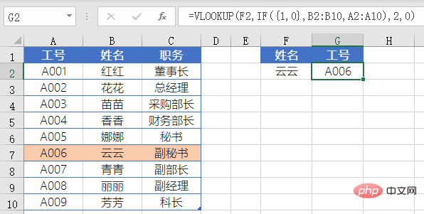
The formula used for G2 is:

=VLOOKUP(F2,IF({1,0},B2:B10,A2:A10),2,0)

We have already talked about the usage of this formula in the previous content, which is to use IF({1,0},B2:B10,A2:A10) to return a name with the name first and the job number first. The resulting multi-row and two-column memory array makes it meet the condition that the query value of the VLOOKUP function is in the first column of the query area, and then use VLOOKUP to query.

This function is relatively complex to use and has low operating efficiency.

Similarly, there is also the use of the CHOOSE function to reconstruct the array, which is to replace the IF({1,0}, part of the formula with CHOOSE({1,2}). This is also a change of the soup without changing the medicine. That’s it.

Method 2

INDEX MATCH combination.

The formula used for G2 is:

=INDEX(A2:A10,MATCH(F2,B2: B10,))

The formula first uses the MATCH function to return the relative position 6 of the name of cell F2 in cells B2:B10, which is the position in this area. Row.

Then use this as the index value of the INDEX function to return the content of the corresponding position from the cell range A2:A10.

This formula is one of the most commonly used query formulas, see It seems cumbersome, but in actual query application, due to its flexible combination, it can complete queries in multiple directions. The operation is flexible and convenient.

Method 3

The invincible LOOKUP function.

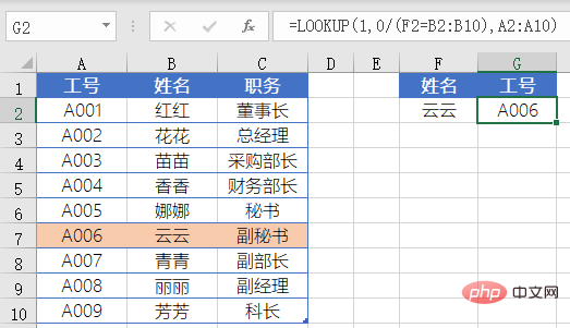
The formula used by G2 is:

=LOOKUP(1,0/(F2=B2:B10),A2:A10)

This is very classic LOOKUP usage.

First use F2=B2:B10 to get a set of logical values, and then divide these logical values ​​by 0 to get a memory array composed of 0 and error values. Then use 1 as the query value, in Query in the memory array.

If the LOOKUP function cannot find the query value, it matches the maximum value in the query area that is less than or equal to the query value, so it matches with the last 0 and returns A2: The value at the same position in A10.

This function is easy to use, powerful, and the formula writing is relatively concise.

If there are multiple results that meet the conditions, the first three formulas will return the first A value that satisfies the condition, and the fourth formula returns the last value that satisfies the condition. You need to pay special attention to this when using it.

Method 4

The fledgling XLOOKUP function .

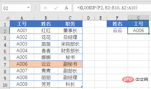
The formula used for G2 is:

=XLOOKUP(F2,B2:B10,A2:A10)

The XLOOKUP function can currently Used in Office 365 and Excel 2021 versions, the first parameter is the content of the query, the second parameter is the area of ​​the query, you only need to select one column in the query area. The third parameter is the content of which column to return, and you only need to select one column That’s it.

The meaning of the formula is to find the name specified in cell F2 in the cell range B2:B10, and return the corresponding name in the cell range A2:A10.

Relevant learning recommendations: excel tutorial

The above is the detailed content of Let's talk about Excel reverse query problem. For more information, please follow other related articles on the PHP Chinese website!