In the previous article "The omnipotent SUMPRODUCT for Excel function learning! 》, we learned the SUMPRODUCT function. Today we are going to talk about three multi-conditional logic functions AND(), OR(), and IF(). Let’s take a look at the explanation together!

For those who are new to functions, you don’t need to understand complex function formulas right away, but you must understand these three multi-conditional logic functions: AND, OR, IF , these three functions can be said to be the most frequently used when writing nested formulas.
Each function is like a calculator. Each calculator has its own special functions. We only need to follow the rules of the calculator and enter data in the corresponding parameter position, and the calculator will automatically complete the function. Special operations. Look at how cumbersome the formula we entered using operators last time is. With functions, we can simplify our thinking process.
1. AND function
In the table shown below, Bottle wants to find out who are the design interns in the design department. This can be done directly using the filtering function of Excel, but today we are going to learn to use functions to solve problems.
Let’s analyze it first. To find a design intern in the design department, two conditions need to be met: “Column D = design” and “column E = design intern”, and Both conditions must be true at the same time (the last tutorial talked about returning true when the result of the comparison operation is true, and the equal sign is also a comparison operator). So how do we use a formula to express that two conditions need to be true at the same time for the result to be true?
You only need to add a * (multiplication sign) between the two conditions, that is (column D = design) * (column E = design intern). When both are true, the multiplication result is 1, which means that he is a design intern in the design department; when any one of them is false, the result is 0, which means he is not a design intern in the design department.
Enter the formula =(D:D= "Design")*(E:E="Design Intern") in cell I2, press Enter and double-click the lower right corner of cell I2 to fill in the formula. You can see that the I3 result is 1, that is, the Hu Tutu in the third row meets the search conditions.

As you can see, if no one tells you the above method, you will need to turn your head twice more to think of it. In fact, we can directly use the AND function to solve the problem, simplifying the thinking process.
AND (parameter 1, parameter 2...) , when parameter 1 and parameter 2 are both true, the result is true.
Select cell I2 and enter the formula in the edit bar =AND (D:D="Design", E:E="Design Intern")

Then press Enter, you can see that the I2 formula result is FALSE. Place the mouse on the lower right corner of cell I2 and double-click to fill in the formula. You can see that only cell I3 is true. The design intern we are looking for is Hu Tutu in row 3.

2. OR function
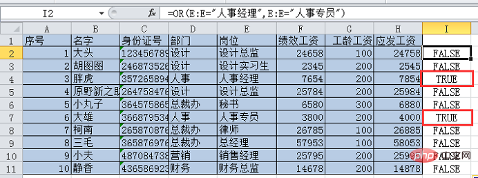
If you want to find the HR specialist or HR manager, just find any Just one person.
The previous bottle used multiplication to ensure that two conditions are met at the same time. Now you can use addition to ensure that any one condition is met.
(Column E=Human Resources Manager) (Column E=Human Resources Specialist), as long as one of them is true, the result of the addition is 1; when both are false, the result is 0.
Enter the formula =(E:E="Personnel Manager") (E:E="Personnel Specialist") in cell I2, press Enter and double-click the lower right corner of cell I2 to fill in formula. You can see that I4 and I7 result in 1.

Similarly, we can also use OR to solve this problem.
OR (parameter 1, parameter 2...) , two parameters, if any one is true, the result is true, if both are false, the result is FALSE.
Enter the formula in cell I2 =OR (E:E="Personnel Manager", E:E="Personnel Specialist"), press Enter, double-click to fill in the formula, the results are as follows , the same lines 4 and 7 are true.

3. IF function
The first two functions are judgment functions and can only judge parameters Whether it is true or false, the output results are only true and false. If the bottle wants to directly output the person's name, it needs to be nested using the IF function.
IF function has three parameters, IF (condition, return value when the condition is true, return value when the condition is false), parameter 1 represents the condition, in the first case above, the condition is the design internship of the design department Health; when the result is true, parameter 2 is returned, which is the corresponding name; when the result is false, parameter 3 is returned, which means that it is not the person you are looking for, so we set the return to blank.
Based on the above analysis, we can write the formula in cell I2
=IF(and(D:D="Design",E:E="Design Internship Raw"),B:B," "), double-click to fill.
In the same way, we can write the formula for the second case.
=IF (OR (E:E="Human Resources Manager", E:E="Human Resources Specialist"),B:B," "), double-click to fill. The results are as follows.

Okay, that’s it for today’s course. In order to test your learning effect, I’ll leave you with a question below.
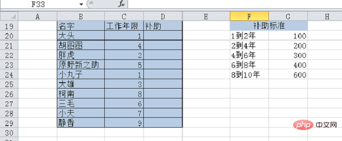
As shown below, the boss is going to distribute a subsidy to everyone, and the subsidy will be distributed according to the number of years of service. So how to write the formula for the subsidy column?

Just use the IF function you learned earlier to solve the problem. Although it is not the easiest way to solve the problem, it can train everyone's hands, especially the formulas require Chinese and English. When switching, and when some characters need to be enclosed in double quotes, errors are most likely to occur. Function experts can also think about whether there is a simpler function that can solve the problem!
Related learning recommendations: excel tutorial
The above is the detailed content of Excel function learning: three multi-conditional logic functions AND(), OR(), IF(). For more information, please follow other related articles on the PHP Chinese website!
 Compare the similarities and differences between two columns of data in excel
 excel duplicate item filter color
 How to copy an Excel table to make it the same size as the original
 Excel table slash divided into two
 Excel diagonal header is divided into two
 Absolute reference input method
 java export excel
 Excel input value is illegal