 Backend Development
 Python Tutorial
 Detailed explanation of Python random forest model examples
Detailed explanation of Python random forest model examples
This article brings you relevant knowledge about Python, which mainly organizes issues related to the random forest model, including an introduction to the ensemble model, the basic principles of the random forest model, and the use of sklearn to implement randomization Let’s take a look at the forest model and other contents. I hope it will be helpful to everyone.

[Related recommendations: Python3 video tutorial ]
1 Introduction to the integrated model
Using an integrated learning model A series of weak learners (also called basic models or base models) learn and integrate the results of each weak learner to obtain better learning results than a single learner.
There are two common algorithms for integrated learning models: Bagging algorithm and Boosting algorithm.
The typical machine learning model of the Bagging algorithm is the random forest model, while the typical machine learning models of the Boosting algorithm are AdaBoost, GBDT, XGBoost and LightGBM models.
1.1 Introduction to Bagging Algorithm
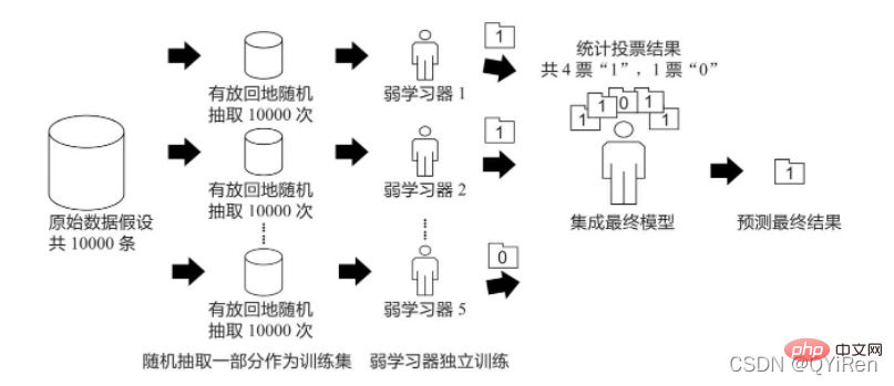
The principle of Bagging algorithm is similar to voting. Each weak learner has one vote. Finally, based on the votes of all weak learners, the principle of "minority obeys the majority" is determined. The final prediction result is shown in the figure below.
Assume that there are 10,000 pieces of original data, and 10,000 data are randomly extracted with replacement to form a new training set (because it is randomly with replacement Backsampling, so a certain piece of data may be sampled multiple times, or a certain piece of data may not be sampled once), each time a training set is used to train a weak learner. In this way, after randomly sampling n times with replacement, at the end of the training, n weak learners trained by different training sets can be obtained. According to the prediction results of these n weak learners, in accordance with the principle of "the minority obeys the majority" , to obtain a more accurate and reasonable final prediction result.
Specifically, in the classification problem, n weak learners are used to vote to obtain the final result, and in the regression problem, n weak learners are used to obtain the final result. The average value of the learner is used as the final result.
1.2 Introduction to Boosting algorithm
The essence of Boosting algorithm is to promote weak learners into strong learners. The difference between it and Bagging algorithm is that Bagging algorithm treats all weak learners equally; The Boosting algorithm will "treat" weak learners differently. In layman's terms, it focuses on "cultivating elites" and "paying attention to mistakes."
"Cultivation of elites" meansafter each round of training, weak learners with more accurate prediction results will be given greater weight, and weak learners with poor performance will be reduced in weight. In this way, in the final prediction, the "excellent model" has a large weight, which is equivalent to it being able to cast multiple votes, while the "general model" can only cast one vote or cannot vote.
"Pay attention to errors" means to change the weight or probability distribution of the training set after each round of training. By increasing the weight of the examples that were wrongly predicted by the weak learner in the previous round, reduce the The weight of the examples correctly predicted by the weak learner in the previous round is used to increase the emphasis of the weak learner on the data that was predicted incorrectly, thus improving the overall prediction effect of the model.
2 Basic principles of the random forest model
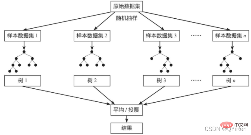
Random Forest (Random Forest) is a classic bagging model, and its weak learner is a decision tree model. As shown in the figure below, the random forest model will randomly sample from the original data set to form n different sample data sets, and then build n different decision tree models based on these data sets, and finally based on the average of these decision tree models value (for regression models) or voting (for classification models) to obtain the final result.
In order to ensure the generalization ability (or general ability) of the model, the random forest model often follows the "data" when building each tree. The two basic principles are "random" and "characteristic randomness".
Random data: Randomly extract data from all data with replacement as training data for one of the decision tree models. For example, there are 1,000 original data, extracted 1,000 times with replacement, to form a new set of data for training a certain decision tree model.
Feature random: If the feature dimension of each sample is M, specify a constant k
Compared with a single decision tree model, the random forest model integrates multiple decision trees, so its prediction results will be more accurate, and it is less likely to cause over-fitting and has stronger generalization ability. .
3 Use sklearn to implement the random forest model
The random forest model can perform both classification analysis and regression analysis. The corresponding models are:
·Random forest classification Model (RandomForestClassifier)
·Random Forest Regression Model (RandomForestRegressor)
The weak learner of the random forest classification model is the classification decision tree model, random forest regression The weak learner of the model is the regression decision tree model.
code show as below.
from sklearn.ensemble import RandomForestClassifier
X = [[1,2],[3,4],[5,6],[7,8],[9,10]]
y = [0,0,0,1,1]

# 设置弱学习器数量为10
model = RandomForestClassifier(n_estimators=10,random_state=123)
model.fit(X,y)

model.predict([[5,5]])

# 输出为:array([0])
4 Case: Stock rise and fall prediction model
4.1 Stock derivative variable generation
This section explains how to use the basic data of stocks to obtain some derivative variable data, such as stock technology Analyze the commonly used moving average indicators: 5-day moving average price MA5 and 10-day moving average price MA10, relative strength indicator RSI, momentum indicator MOM, exponential moving average EMA, moving average similarity and difference MACD, etc.
4.1.1 Obtain basic stock data
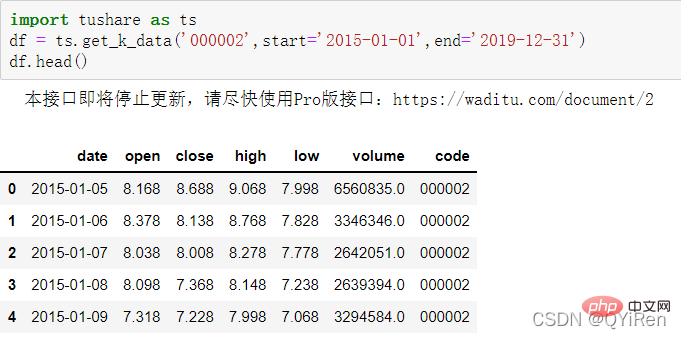
First use the get_k_data() function to obtain the basic stock data from 2015-01-01 to 2019-12-31. The code is as follows.
The first 5 rows of data are shown in the figure below. The missing data is holiday (non-trading day) data.
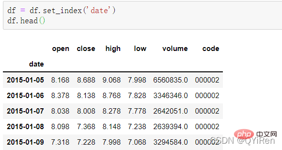
Use the set_index() function to set the date column to the row index , the code is as follows.
4.1.2 Generating simple derived variables
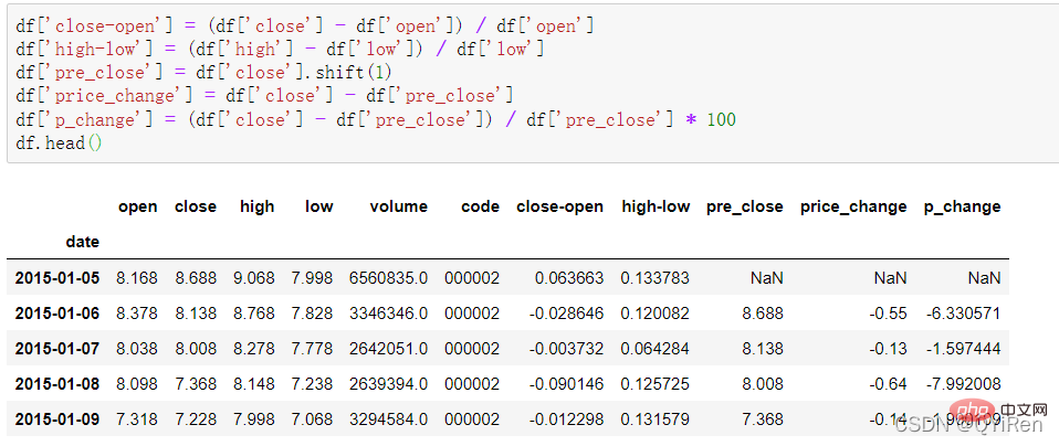
Some simple derived variable data can be generated through the following code.
close-open means (closing price - opening price)/opening price;
high-low means (highest price - lowest price)/lowest price;
pre_close represents yesterday's closing price. Use shift(1) to move all the data in the close column down 1 row and form a new column. If it is shift(- 1) means moving up 1 line;
price_change represents today's closing price - yesterday's closing price, that is, the change in stock price on that day;
p_change represents the percentage change in stock price on that day, also known as It is the increase or decrease of the stock price on that day.
4.1.3 Generate moving average indicator MA value
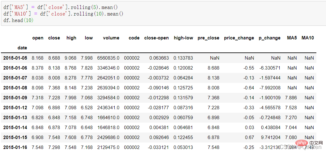
The 5-day moving average and 10-day moving average of the stock price can be generated through the following code.
Note: The use of rolling function
##Among them, MA means moving average, " "Average" refers to the arithmetic mean of the closing prices of the last n days, and "moving" means that the price data of the last n days are always used in the calculation.
For example: Calculation of MA5When calculating data like MA5, because the amount of data in the first 4 days is insufficient, the moving average corresponding to these 4 days cannot be calculated, so a null value NaN will be generated. Usually, the dropna() function is used to delete null values to avoid problems caused by null values in subsequent calculations. The code is as follows.According to the above data, the MA5 value of No. 5 is (1.2+1.4+1.6+1.8+2.0 )/5=1.6, and the MA5 value of No. 6 is (1.4+1.6+1.8+2.0+2.2)/5=1.8, and so on. The moving average of stock prices over a period of time is connected into a curve, which is the moving average. Similarly, MA10 is the average stock price of the previous 10 days from the day of calculation.
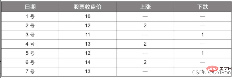
#You can see that the rows before the 16th are deleted. 4.1.4 Use the TA-Lib library to generate the relative strength indicator RSI valueThe relative strength indicator RSI value can be generated through the following code.
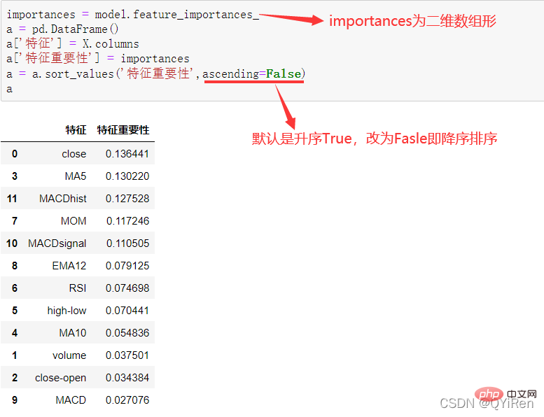
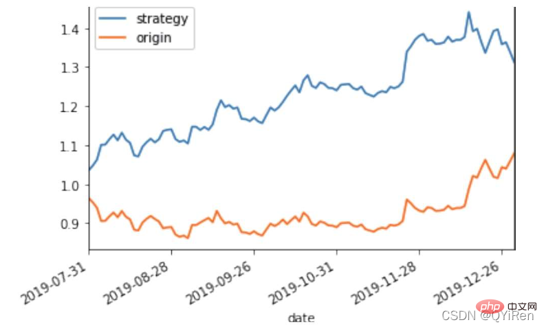
RSI value can reflect the strength of the stock price increase relative to the decline in the short term, helping us make better judgments The rising and falling trend of stock prices. The greater the RSI value, the stronger the upward trend is relative to the downward trend, and conversely, the weaker the upward trend is relative to the downward trend. The calculation formula of RSI value is as follows. Example: Based on the data in the above table, take N=6 , it can be obtained that the 6-day average rising price is (2+2+2)/6=1, and the 6-day average falling price is (1+1+1)/6=0.5, so the RSI value is (1/(1+0.5))×100=66.7. Normally, the RSI value is between 20 and 80. If it exceeds 80, it is overbought, if it is below 20, it is oversold. If it is equal to 50, it is considered that the power of buyers and sellers is equal. For example, if the stock price rises for 6 consecutive days, the average falling price on the 6th day will be 0, and the RSI value on the 6th day will be 100. This indicates that the stock buyer is in a very strong position at this time, but investors are also reminded to be wary that this may also be an excessive period. In the buying state, you need to prevent the risk of stock price falling. The momentum indicator MOM value can be generated through the following code. MOM is the abbreviation of momentum, which reflects the rate of rise and fall of stock prices over a period of time, calculation formula as follows. Example: Suppose you want to calculate the MOM value of No. 6, In the previous code, the parameter timeperiod is set to 5, then you need to subtract the closing price of No. 1 from the closing price of No. 6, that is, the MOM value of No. 6 is 2.2-1.2=1. Similarly, the MOM value of No. 7 is 2.4-1.4=1. Connecting the MOM values for consecutive days forms a curve that reflects the rise and fall of the stock price. You can generate exponential moving average EMA through the following code. EMA is a moving average weighted in exponential decreasing order, and is analyzed based on the calculation results. is used to determine changes in the future trend of the stock price. trend. The calculation formula of EMA is as follows. Among them, EMAtoday is the EMA value of the day; Pricetoday is the closing price of the day; EMAyesterday is yesterday's EMA value; α is the smoothing index, generally The value is 2/(N+1), N represents the number of days, when N is 6, α is 2/7, and the corresponding EMA is called EMA6, which is a 6-day exponential moving average. The formula continues to recurse until the first EMA value appears (the first EMA value is usually the average of the first 5 numbers). Example: EMA6 The first EMA value is taken as the average of the first 5 numbers, so there is no EMA value in the first 5 days; The EMA value on No. 6 is the first EMA value, which is the average of the previous five days, that is, 1; the EMA value on No. 7 is the second EMA value. The calculation process is as follows. You can generate MACD values for the Moving Average Convergence and Divergence through the following code . MACD is a commonly used indicator in the stock market. It is a derivative variable based on the EMA value. The calculation method is relatively complicated. Interested readers can learn. Here you only need to know that MACD is a trend indicator, and its changes represent changes in market trends. MACD at different K-line levels represents the buying and selling trend in the current level cycle. 首先强调最核心的一点:应该是用当天的股价数据预测下一天的股价涨跌情况,所以目标变量y应该是下一天的股价涨跌情况。为什么是用当天的股价数据预测下一天的股价涨跌情况呢?这是因为特征变量中的很多数据只有在当天交易结束后才能确定(例如,收盘价close只有收盘了才有),所以当天正在交易时的股价涨跌情况是无法预测的,而等到收盘时尽管所需数据齐备,但是当天的股价涨跌情况已成定局,也就没有必要预测了,所以是用当天的股价数据预测下一天的股价涨跌情况。 第2行代码中使用了NumPy库中的where()函数,传入的3个参数的含义分别为判断条件、满足条件的赋值、不满足条件的赋值。其中df['price_change'].shift(-1)是利用shift()函数将price_change(股价变化)这一列的所有数据向上移动1行,这样就获得了每一行对应的下一天的股价变化。因此,这里的判断条件就是下一天的股价变化是否大于0,如果大于0,说明下一天股价涨了,则y赋值为1;如果不大于0,说明下一天股价不变或跌了,则y赋值为-1。预测结果就只有1或-1两种分类。 这里需要注意的是,划分要按照时间序列进行,而不能用train_test_split()函数进行随机划分。这是因为股价的变化趋势具有时间性特征,而随机划分会破坏这种特征,所以需要根据当天的股价数据预测下一天的股价涨跌情况,而不能根据任意一天的股价数据预测下一天的股价涨跌情况。 将前90%的数据作为训练集,后10%的数据作为测试集,代码如下。 设置模型参数:决策树的最大深度max_depth设置为3,即每个决策树最多只有3层;弱学习器(即决策树模型)的个数n_estimators设置为10,即该随机森林中共有10个决策树;叶子节点的最小样本数min_samples_leaf设置为10,即如果叶子节点的样本数小于10则停止分裂;随机状态参数random_state的作用是使每次运行结果保持一致,这里设置的数字123没有特殊含义,可以换成其他数字。 用predict_proba()函数可以预测属于各个分类的概率,代码如下。 通过如下代码可以查看整体的预测准确度。 打印输出score为0.40,说明模型对整个测试集中约40%的数据预测正确。这一预测准确度并不算高,也的确符合股票市场千变万化的特点。 通过如下代码可以分析各个特征变量的特征重要性。 由图可知,当日收盘价close、MA5、MACDhist相关指标等特征变量对下一天股价涨跌结果的预测准确度影响较大。 前面已经评估了模型的预测准确度,不过在商业实战中,更关心它的收益回测曲线(又称为净值曲线),也就是看根据搭建的模型获得的结果是否比不利用模型获得的结果更好。 可视化结果如下图所示。图中上方的曲线为根据模型得到的收益率曲线,下方的曲线为股票本身的收益率曲线,可以看到,利用模型得到的收益还是不错的。 要说明的是,这里讲解的量化金融内容比较浅显,搭建的模型过于理想化,真正的股市是错综复杂的,股票交易也有很多限制,如不能做空、不能T+0交易,还要考虑手续费等因素。 随机森林模型是一种非常重要的集成模型,它集成了决策树模型的众多优点,又规避了决策树模型容易过度拟合等缺点,在实战中应用较为广泛。 【相关推荐:Python3视频教程 】
4.1.5 Use the TA-Lib library to generate the momentum indicator MOM value


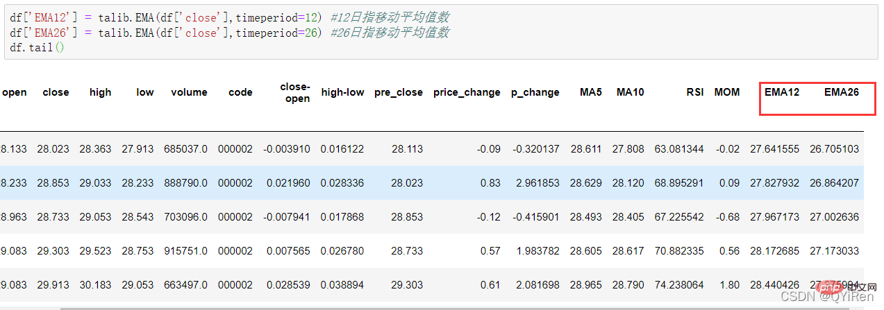
4.1.6 Use TA-Lib library to generate exponential moving average EMA


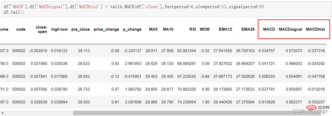
4.1.7 Use the TA-Lib library to generate MACD values for the Moving Average Convergence and Divergence
4.2 模型搭建
4.2.1 引入需要搭建的库
# 导入相关库
import tushare as ts
import numpy as np
import pandas as pd
import talib
import matplotlib.pyplot as plt
from sklearn.ensemble import RandomForestClassifier
from sklearn.metrics import accuracy_score
4.2.2 获取数据
# 1.股票基本数据获取
import tushare as ts
df = ts.get_k_data('000002',start='2015-01-01',end='2019-12-31')
df = df.set_index('date')

# 2.简单衍生变量数据构造
df['close-open'] = (df['close'] - df['open']) / df['open']
df['high-low'] = (df['high'] - df['low']) / df['low']
df['pre_close'] = df['close'].shift(1)
df['price_change'] = df['close'] - df['pre_close']
df['p_change'] = (df['close'] - df['pre_close']) / df['pre_close'] * 100

# 3.移动平均线相关数据构造
df['MA5'] = df['close'].rolling(5).mean()
df['MA10'] = df['close'].rolling(10).mean()
df.dropna(inplace=True)

# 4.通过TA-Lib库构造衍生变量数据
df['RSI'] = talib.RSI(df['close'],timeperiod=12)
df['MOM'] = talib.MOM(df['close'],timeperiod=5)
df['EMA12'] = talib.EMA(df['close'],timeperiod=12) #12日指移动平均值数
df['EMA26'] = talib.EMA(df['close'],timeperiod=26) #26日指移动平均值数
df['MACD'],df['MACDsignal'],df['MACDhist'] = talib.MACD(df['close'],fastperiod=6,slowperiod=12,signalperiod=9)
df.dropna(inplace=True)4.2.3 提取特征变量和目标变量
X = df[['close','volume','close-open','MA5','MA10','high-low','RSI','MOM','EMA12','MACD','MACDsignal','MACDhist']]
y = np.where(df['price_change'].shift(-1) > 0,1,-1)
4.2.4 划分训练集和测试集
X_length = X.shape[0]
split = int(X_length * 0.9)
X_train,X_test = X[:split],X[split:]
y_train,y_test = y[:split],y[split:]
4.2.5 模型搭建
model = RandomForestClassifier(max_depth=3,n_estimators=10,min_samples_leaf=10,random_state=123)
model.fit(X_train,y_train)
4.3 模型评估与使用
4.3.1 预测下一天的股价涨跌情况
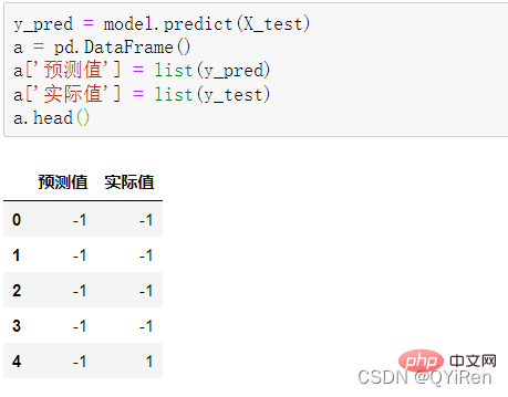
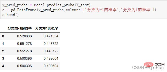
4.3.2 模型准确度评估
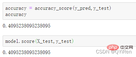
4.3.3 分析特征变量的特征重要性
4.4 参数调优
from sklearn.model_selection import GridSearchCV
parameters={'n_estimators':[5,10,20],'max_depth':[2,3,4,5,6],'min_samples_leaf':[5,10,20,30]}
new_model = RandomForestClassifier(random_state=123)
grid_search = GridSearchCV(new_model,parameters,cv=6,scoring='accuracy')
grid_search.fit(X_train,y_train)
grid_search.best_params_

# 输出
# {'max_depth': 5, 'min_samples_leaf': 20, 'n_estimators': 5} 4.5 收益回测曲线绘制
# 在测试数据上添加一列,预测收益
X_test['prediction'] = model.predict(X_test)

# 计算每天的股价变化率
X_test['p_change'] = (X_test['close'] - X_test['close'].shift(1)) / X_test['close'].shift(1)

# 计算累积收益率
# 例如,初始股价是1,2天内的价格变化率为10%
# 那么用cumprod()函数可以求得2天后的股价为1×(1+10%)×(1+10%)=1.21
# 此结果也表明2天的收益率为21%。
X_test['origin'] = (X_test['p_change'] + 1).cumprod()

# 计算利用模型预测后的收益率
X_test['strategy'] = (X_test['prediction'].shift(1) * X_test['p_change'] + 1).cumprod()

X_test[['strategy','origin']].dropna().plot()
# 设置自动倾斜
plt.gcf().autofmt_xdate()
plt.show()
The above is the detailed content of Detailed explanation of Python random forest model examples. For more information, please follow other related articles on the PHP Chinese website!

Hot AI Tools

Undresser.AI Undress
AI-powered app for creating realistic nude photos

AI Clothes Remover
Online AI tool for removing clothes from photos.

Undress AI Tool
Undress images for free

Clothoff.io
AI clothes remover

Video Face Swap
Swap faces in any video effortlessly with our completely free AI face swap tool!

Hot Article

Hot Tools

Notepad++7.3.1
Easy-to-use and free code editor

SublimeText3 Chinese version
Chinese version, very easy to use

Zend Studio 13.0.1
Powerful PHP integrated development environment

Dreamweaver CS6
Visual web development tools

SublimeText3 Mac version
God-level code editing software (SublimeText3)

Hot Topics
 1387
1387
 52
52
 Is the vscode extension malicious?
Apr 15, 2025 pm 07:57 PM
VS Code extensions pose malicious risks, such as hiding malicious code, exploiting vulnerabilities, and masturbating as legitimate extensions. Methods to identify malicious extensions include: checking publishers, reading comments, checking code, and installing with caution. Security measures also include: security awareness, good habits, regular updates and antivirus software.
 How to run programs in terminal vscode
Apr 15, 2025 pm 06:42 PM
In VS Code, you can run the program in the terminal through the following steps: Prepare the code and open the integrated terminal to ensure that the code directory is consistent with the terminal working directory. Select the run command according to the programming language (such as Python's python your_file_name.py) to check whether it runs successfully and resolve errors. Use the debugger to improve debugging efficiency.
 Can vs code run in Windows 8
Apr 15, 2025 pm 07:24 PM
VS Code can run on Windows 8, but the experience may not be great. First make sure the system has been updated to the latest patch, then download the VS Code installation package that matches the system architecture and install it as prompted. After installation, be aware that some extensions may be incompatible with Windows 8 and need to look for alternative extensions or use newer Windows systems in a virtual machine. Install the necessary extensions to check whether they work properly. Although VS Code is feasible on Windows 8, it is recommended to upgrade to a newer Windows system for a better development experience and security.
 Can visual studio code be used in python
Apr 15, 2025 pm 08:18 PM
VS Code can be used to write Python and provides many features that make it an ideal tool for developing Python applications. It allows users to: install Python extensions to get functions such as code completion, syntax highlighting, and debugging. Use the debugger to track code step by step, find and fix errors. Integrate Git for version control. Use code formatting tools to maintain code consistency. Use the Linting tool to spot potential problems ahead of time.
 Choosing Between PHP and Python: A Guide
Apr 18, 2025 am 12:24 AM
PHP is suitable for web development and rapid prototyping, and Python is suitable for data science and machine learning. 1.PHP is used for dynamic web development, with simple syntax and suitable for rapid development. 2. Python has concise syntax, is suitable for multiple fields, and has a strong library ecosystem.
 Can vscode be used for mac
Apr 15, 2025 pm 07:36 PM
VS Code is available on Mac. It has powerful extensions, Git integration, terminal and debugger, and also offers a wealth of setup options. However, for particularly large projects or highly professional development, VS Code may have performance or functional limitations.
 Can vscode run ipynb
Apr 15, 2025 pm 07:30 PM
The key to running Jupyter Notebook in VS Code is to ensure that the Python environment is properly configured, understand that the code execution order is consistent with the cell order, and be aware of large files or external libraries that may affect performance. The code completion and debugging functions provided by VS Code can greatly improve coding efficiency and reduce errors.
 Golang vs. Python: Concurrency and Multithreading
Apr 17, 2025 am 12:20 AM
Golang is more suitable for high concurrency tasks, while Python has more advantages in flexibility. 1.Golang efficiently handles concurrency through goroutine and channel. 2. Python relies on threading and asyncio, which is affected by GIL, but provides multiple concurrency methods. The choice should be based on specific needs.


