This article brings you relevant knowledge about excel, which mainly organizes the related issues of function combination. The role and function of a single function are relatively single. When solving practical problems , often requires multiple functions to be nested. Let’s take a look at them together. I hope it will be helpful to everyone.

Related learning recommendations: excel tutorial
The role and function of a single function are relatively simple. When solving practical problems , often require multiple functions to be nested. Today I will share with you some commonly used function nesting combinations. Once you are familiar with the use of these nested functions, it is still possible to improve efficiency.
One of the query functions with the highest appearance rate.
Use the MATCH function to locate the position of the query value, and then use the INDEX function to return the content of the specified position in the specified area. The combination of the two can achieve all-round querying from top to bottom, left and right.
Application example:
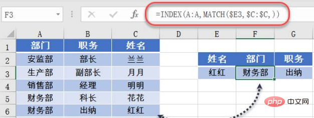
As shown in the figure below, querying the department and position based on the name is the legendary reverse query.

F3 cell formula is:
=INDEX(A:A,MATCH($E3,$C:$C,))
MATCH to find the precise location of cell E3 in column C: Old IN, Honghong is in the 6th room.
Next, INDEX finds the 6th cell from column A based on the clues provided by MATCH: Oh, this is the window of Honghong’s house, let’s start——
Used to calculate the minimum value of specified conditions.
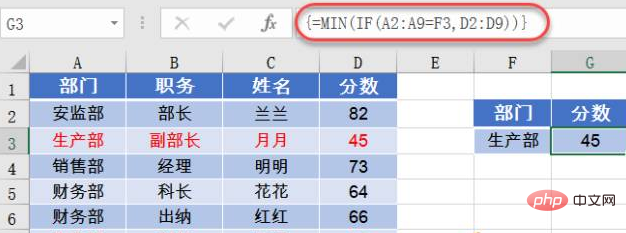
As shown in the figure below, the minimum score of the production department is calculated.

G3 cell can use array formula:
=MIN(IF(A2:A9=F3,D2:D9))
First use the IF function to determine whether the department in column A is equal to the department specified by F3. If the condition is true, return the score corresponding to column D, otherwise return the logical value FALSE:
{FALSE;45;FALSE;FALSE; FALSE;66;FALSE;72}
Next, use the MIN function to calculate the minimum value.
The MIN function has a feature that it can automatically ignore logical values, so it will only calculate the numerical part, and finally get the lowest score of the specified department.
Note that since multiple calculations are performed, you must press the Shift ctrl Enter key when entering the formula.
is often used for data queries with an uncertain number of columns.
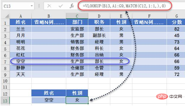
As shown in the figure below, the corresponding item must be queried in the data table based on the name of cell B13.

The formula in cell C13 is:
=VLOOKUP(B13,A1:G9,MATCH(C12,1:1,),0)
If the number of columns in the data table is very large, when using the VLOOKUP function, you still need to calculate on your fingers which column the queried item is in the data table, which is really troublesome.
Okay now, first use the MATCH function to query the column in which the item is located, and then the VLOOKUP function returns the content of the corresponding column based on the information provided by the MATCH function.
Calculate how many items there are in a cell.
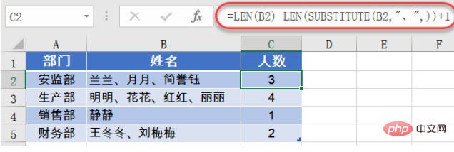
As shown in the figure below, the number of people in each department must be calculated.

This kind of table must be familiar to everyone. Multiple names are in one cell, and each name is separated by a comma.
C2 cell formula is:
=LEN(B2)-LEN(SUBSTITUTE(B2,”,”,)) 1
First use the LEN function to calculate B The character length of the column cell, and then use the SUBSTITUTE function to replace all commas and calculate the replaced character length.
Subtract the replaced character length from the character length to get the number of commas in the cell.
Next, add 1 to get the actual number of people, you know.
is often used to extract and convert date strings.
As shown in the figure below, the date and month of birth must be extracted based on the ID number in column B.

The formula in cell C2 is:
=–TEXT(MID(B2,7,8),”0-00-00″)
The MID function is used to extract a specific number of strings starting from a specified position in the string.
MID(B2,7,8) starts from the 7th digit of cell B2 and extracts 8 digits. The result is:
19751226
Then use the TEXT function , change this string into the pattern of "0-00-00", and the result is "1975-12-26".
At this time, the date already looks like it, but it is still text type, so two negative signs are added, which is to calculate the negative number of the negative number. After such a toss, it becomes a real date. Sequenced.
Related learning recommendations: excel tutorial
The above is the detailed content of Summary and sharing of common function combinations in Excel. For more information, please follow other related articles on the PHP Chinese website!
 Compare the similarities and differences between two columns of data in excel
 excel duplicate item filter color
 How to copy an Excel table to make it the same size as the original
 Excel table slash divided into two
 Excel diagonal header is divided into two
 Absolute reference input method
 java export excel
 Excel input value is illegal


