This article brings you relevant knowledge about excel, which mainly organizes the related issues of querying data under any conditions. How to implement data query? The left side is the employee information table, and the right side is the query. Area, I hope that by entering any name or any department in G4, all records that meet the conditions can be extracted on the right side. Let’s take a look at it. I hope it will be helpful to everyone.

Related learning recommendations: excel tutorial
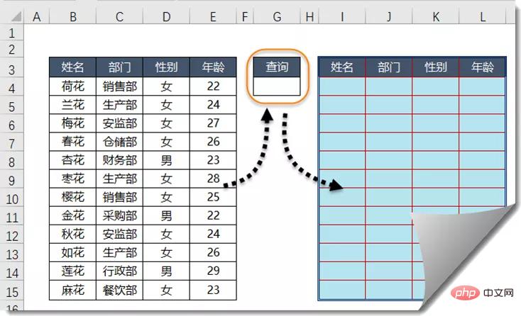
To share a content related to data query, first look at the data source:

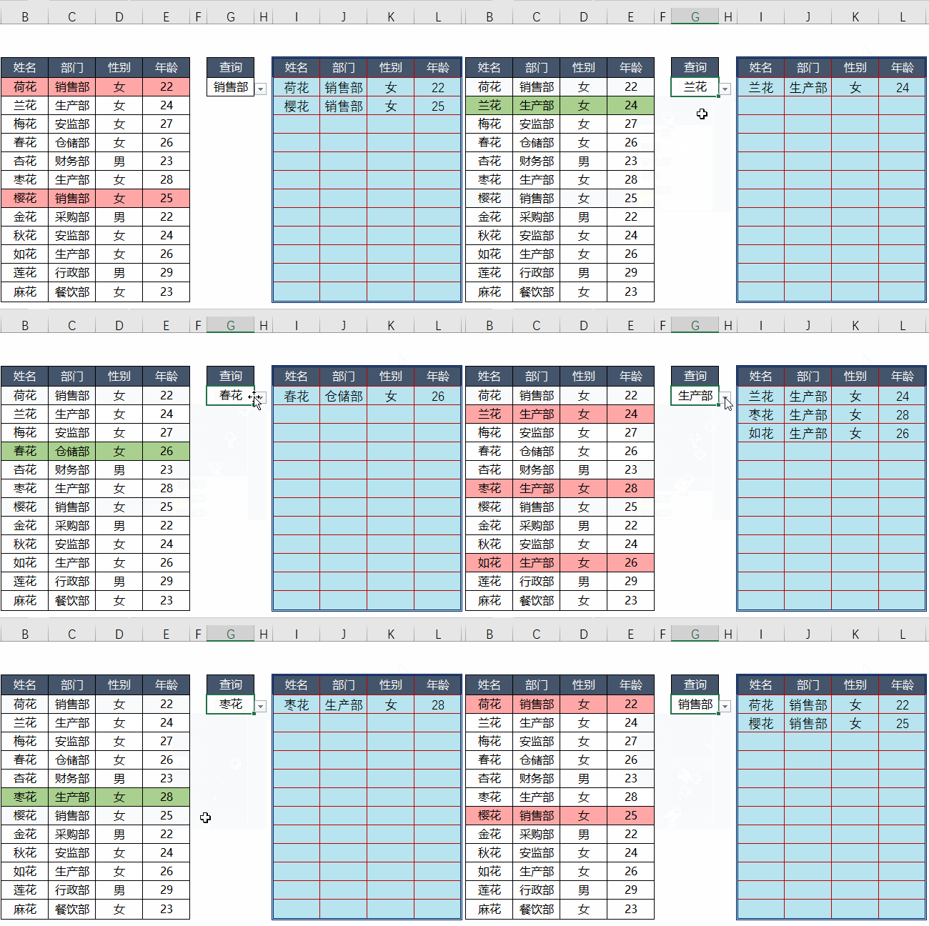
The left side is the employee information table, and the right side is the query area. If you want to enter any name or any department in G4, you can extract all records that meet the conditions on the right side.

#To achieve such a data extraction effect, it is actually very simple. Next, let’s take a look at the specific steps.
Enter the content to be queried in cell G4, such as Sales Department.
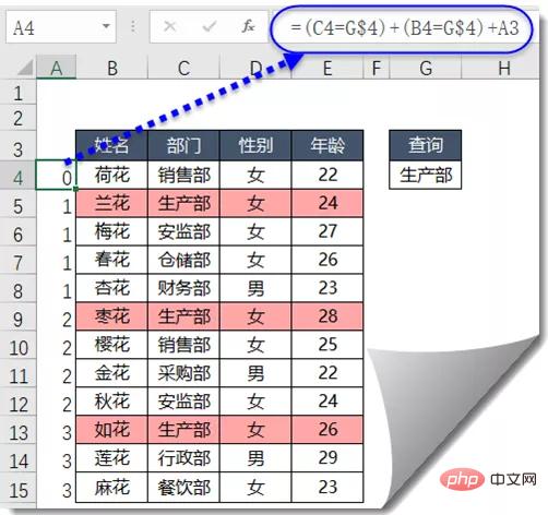
On the left side of the first row of data, in this case cell A4, enter the following formula and drag down:
=(C4=G $4) (B4=G$4) A3

What does the formula mean?
If the department in cell C4 is equal to the department to be queried by G4, or the name in cell B4 is equal to the name to be queried in cell G4, add 1 to the previous cell. Otherwise, it remains the content of the previous cell.
Observe the effect of the drop-down formula. You can see that as long as the department name in column C is equal to the department in cell G4, the result is exactly a series of increasing serial numbers 1...2...3...
What are these serial numbers used for? Don't worry, look down.
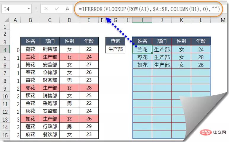
Enter the formula in cell I4, copy it to the right and down, and you can get the query results:
=IFERROR(VLOOKUP(ROW(A1), $A:$E,COLUMN(B1),0),"")

What does this formula mean?
The protagonist here is the VLOOKUP function. The content to be queried is ROW(A1). The function of ROW is to return the row number where the parameter is located. The result obtained here is the row number of A1 - 1. When the formula When copied downward, it will become ROW(A2), ROW(A3)..., and the result is the increasing sequence number 1, 2, 3... starting from 1.
In other words, the search content of the VLOOKUP function is different in different rows. In the fourth row, the search content is 1, and when the formula reaches the fifth row, the query content is 2.
Let’s take a look at the area queried by the VLOOKUP function? $A:$E, this writing method represents the entire column area of columns A~E, and uses absolute references.
Speaking of which, some friends already know what the serial numbers we obtained using the formula are used for. Yes, they are used to assist VLOOKUP queries.
The characteristic of the previous sequence number is that every time it encounters a record that meets the conditions, the sequence number is added by 1, and the content to be queried by VLOOKUP is the sequence number 1, 2, 3...
Let’s look at COLUMN What is (B1) used for? Its function is similar to the ROW function. It returns the column number of the parameter, COLUMN(B1), and the result is the column number 2 of B1. When the formula is copied to the right, it will turn into COLUMN (C1), COLUMN (D1)..., and the result is the incremental serial number starting from 2, 2, 3, 4...
The obtained serial number is then given to the VLOOKUP function When Xiaosan, no, it is used as the third parameter, used to specify which column in the query area is returned.
When the formula is in column I, the content of the second column of the query area is returned. If the formula is copied to the right to column J, the content of the third column of the query area is returned, and so on.
My friends may say that there are so many repeated serial numbers in column A. It doesn't matter, because the VLOOKUP function has a characteristic that if there are multiple records that meet the conditions, only the first one will be returned. So when you query 1 in cell I4, you get the name Orchid corresponding to serial number 1, and when you query 2 in cell I5, you get the name Zaohua corresponding to serial number 2...
The outermost IFERROR is Qian What is it used for? She is used to shield VLOOKUP from error values.
Because the query sequence number in each row of VLOOKUP is different, when the formula keeps pulling down, the sequence number will continue to increase. When the query sequence number does not appear in column A, it means that there are not so many records on the left If the content meets the conditions, the formula will return an error value. Therefore, we use the IFERROR function to turn the error value into empty text.
Related learning recommendations: excel tutorial
The above is the detailed content of Easily check data under any conditions in Excel. For more information, please follow other related articles on the PHP Chinese website!
 Compare the similarities and differences between two columns of data in excel
 excel duplicate item filter color
 How to copy an Excel table to make it the same size as the original
 Excel table slash divided into two
 Excel diagonal header is divided into two
 Absolute reference input method
 java export excel
 Excel input value is illegal


