In the previous article "How to deal with common complications in learning Excel pivot tables", we learned how to deal with common complications in pivot tables. Today we continue to learn pivot tables. . Pivot table is one of the very important tools in Excel. It saves us a lot of time. Many times you work overtime, maybe because you don't know how to use it. Today I will share with you the third tutorial on pivot tables. It mainly explains how to sort Excel pivot tables and how to insert excel pivot table formulas. Take a look below!

I have previously posted two tutorials on excel pivot tables. I believe everyone already has a general understanding of pivot tables, right? Usually we use pivot tables to summarize data. As soon as we drag and drop the fields, 80% of the work of summarizing the data is completed. It is so convenient! So today we will deal with the remaining 20% of the work~
1. Sort the pivot table
As shown in the figure In the table, the data needs to be statistically calculated to calculate the proportion of the quantity and amount received by each person in each department, and it can be filtered by month. I believe that friends who have read the first two tutorials will be able to operate it.
I won’t go into details here. The results of the pivot table are as follows. In this article, we will continue to learn how to sort Excel pivot tables.

1. Sorting by single key field
Now you need to arrange the collection quantity in order from high to low. Right-click any cell in the collection quantity column and click "Sort" - "Descending".

You can see that the summary quantity of each department is arranged in descending order, but the number of people in each department is not arranged in descending order.

Right-click any cell in the position column and select "Sort" - "Other Sorting Options".

In the pop-up dialog box, click "Sort Descending" - "Receive Quantity". Click OK.

#You can see at this point that the number of people in each department has also been sorted in descending order.

2. Sorting by multiple key fields
Our previous requirement is just to sort the quantity received, then if When the quantities are the same, what about the descending order of amounts?
In order to show you more intuitively, we first cancel the classification and summary. Click on the pivot table and click "Design" - "Subtotals" - "Do not show subtotals" in the floating tab. Then delete the "Department" and "Position" fields. The results are as follows.

Right-click in the collection quantity column and click "Sort" - "Descending Order". The results are as follows.

When the received quantities are the same, sort them in descending order by amount. Right-click in the amount column and select descending order. The results are as follows.

#You will find that the amount is sorted in descending order, but the collection amount column is disrupted again. Because the pivot table is refreshed every time it is sorted, the results of the last sort will not be saved.
Right-click in the name column and select "Sort" - "Other Sorting Options". Click "Other Options" in the pop-up dialog box.

Uncheck "Automatically sort every time the report is updated". Click OK.

At this time, set the amount and received quantity in descending order to get the correct result. As shown below, the received quantities are arranged in descending order. When the received quantities are the same, they are arranged in descending order according to the amount.

3. Manually enter the sorting
table as shown below. We first create a pivot table.

The pivot table is as shown below, we need to sort the department column.

#If you directly right-click to sort in ascending order, the result is as follows. The Chinese characters are sorted in ascending order of pinyin, which is not the result we want.

In fact, we directly click on the first cell, enter "Market 1" and press Enter, and the department columns will be sorted. As follows.

4. Set custom sorting
In the first three methods, we first create a pivot table and then sort the data. To sort, we can actually set the sorting rules in advance.
Click "File"-"Options" and the dialog box shown below will pop up.

Click "Advanced" - "General" - "Edit Custom List".

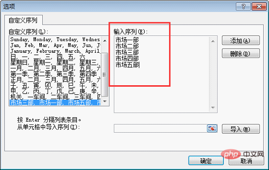
Enter the sequence on the right, press Enter and line feed.

Click Add and you can see it in the custom sequence on the left. Click OK.
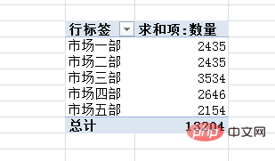
At this time, we select the data area of the previous case, insert the pivot table, drag in the fields, and you will see that the first column of the pivot table has been automatically sorted. .

2. Insert formulas into the Pivot Table
It is also very convenient to use formulas in the Pivot Table , we still use the first case data as a demonstration.
The company stipulates that 0.3% of the total amount of materials received by each person within a year must be deducted from each person's salary.
Click on the pivot table and click "Options" - "Fields, Items, and Sets" - "Calculated Fields" in the floating tab.
Enter "deduction amount" after the name.
Then enter the equal sign after the formula, click the field "Amount" below, and click "Insert Field", then "Amount" will appear after the formula.
After entering the complete formula, click OK.
#You will see a column automatically inserted behind the pivot table, and the amount that each person needs to deduct has been calculated.
After reading today’s tutorial, you are no longer as unfamiliar with pivot tables as you were at first, right? Being proficient in using the pivot table and giving full play to the role of each tool can bring great convenience to our work. We must follow the instructions again!
Related learning recommendations: excel tutorial
The above is the detailed content of 4 ways to learn sorting and insert formulas in Excel pivot tables. For more information, please follow other related articles on the PHP Chinese website!
 Compare the similarities and differences between two columns of data in excel
 excel duplicate item filter color
 How to copy an Excel table to make it the same size as the original
 Excel table slash divided into two
 Excel diagonal header is divided into two
 Absolute reference input method
 java export excel
 Excel input value is illegal


