
 Topics
excel
Excel function learning: Let's talk about how to use countif() (detailed case explanation)
Topics
excel
Excel function learning: Let's talk about how to use countif() (detailed case explanation)
Excel function learning: Let's talk about how to use countif() (detailed case explanation)

In the previous article "Excel function learning: How to quickly count working days, take a look at these two functions! 》, we learned two working day functions. Today we are going to learn countif() and share 5 cases of countif function checking for duplicates. Come and take a look!

There are some very classic function combinations in Excel. The more familiar ones are the INDEX-MATCH combination and the INDEX-SMALL-IF-ROW combination (also called Tiger Balm). combination), of course there are many other combinations. The combination shared today is also very useful. Below, we will use four common questions to let everyone witness the wonderful moments brought by this combination. Of course, we still need to get to know the two people today. Two protagonists: COUNTIF and IF, two functions that everyone is very familiar with.
How to use the COUNTIF function: COUNTIF (range, condition), the function can get the number of times that data that meets the conditions appears in the range. Simply put, this function is used for conditional counting;
Usage of the IF function: IF (condition, result that satisfies the condition, result that does not satisfy the condition), in one sentence, if you give IF a condition (the first parameter), when the condition is established, it will return a result (the second parameter) parameter), when the condition is not met, another result is returned (the third parameter).
Regarding the basic usage of these two functions, I have talked about it many times in previous tutorials, so I won’t go into details here. Let’s take a look at the first problem that occurred after the two of them met: When checking orders The question on
Assume that column A is all the order numbers, and column D is the order number that has been shipped. Now you need to mark the shipped orders in column B (in order to prevent everyone from being dazzled, The arrows only point out two corresponding order numbers):
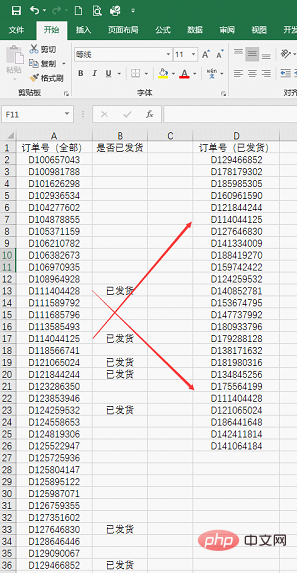
I think you must be familiar with this question. This question is in the reconciliation I use it often, and maybe some friends can’t wait to shout VLOOKUP. In fact, the formula in column B is like this:
=IF(COUNTIF(D:D,A2)> 0,"shipped","")
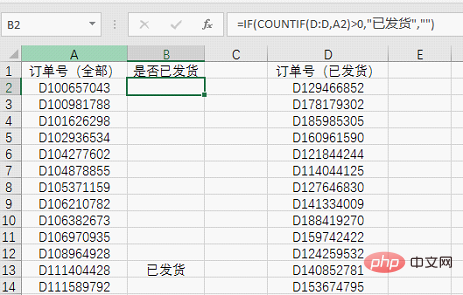
First use COUNTIF to make statistics and see that the order number in cell A2 is in D The column appears several times. If it does not appear, it means it has not been shipped. Otherwise, it means it has been shipped.
Therefore, use COUNTIF(D:D,A2)>0 as the condition of IF. If the order appears in column D (the number of occurrences is greater than 0), then "shipped" is returned (note that Chinese characters must be added quotes), otherwise it returns blank (two quotes represent blank).
Now that you understand the first question, let’s look at the second question: COUNTIF to check duplicate cases: How to find duplicate orders
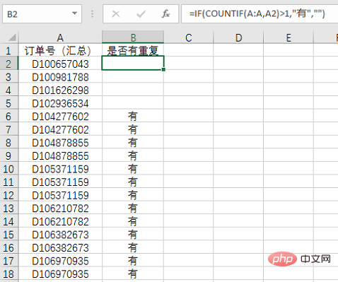
Column A comes from multiple After summarizing the order statistics table registered by the clerk, it is found that some are duplicates (for the convenience of viewing, you can sort the order numbers first). Now you need to mark the duplicate orders in column B:
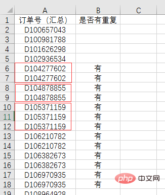
This is also a problem with a very high ranking rate, and the solution is also very simple. The formula in column B is:
=IF(COUNTIF(A :A,A2)>1,"有","")
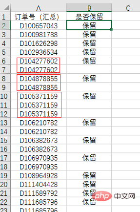
This problem seems quite troublesome at first glance. In fact, it can be achieved by slightly modifying the formula of question 2: =IF(COUNTIF($ A$2:A2,A2)=1,"Keep","")
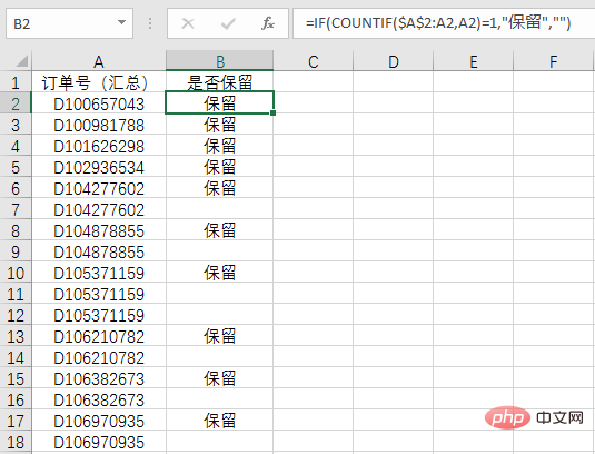
Note the COUNTIF here, the range is no longer The entire column is $A$2:A2. This way of writing will change the statistical range as the formula is pulled down. The result is as follows:
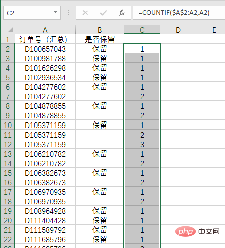
It is not difficult to see that the order number with a result of 1 is the first time it appears, which is also the information we need to retain, so when it is used as a condition, equal to 1 is used.
The first three questions are all related to the order number, and the last question is related to Supplier Assessment, which is the key issue that determines whether the contract can be renewed.
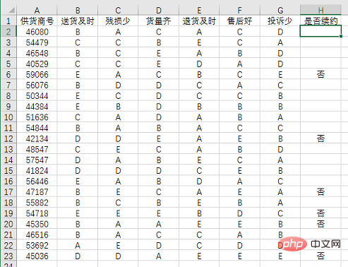
According to company regulations, there are six assessment indicators for each supplier. A is the best and E is the worst. If there are two or more E's in the six indicators, the contract will not be renewed. :
The rules are relatively simple. Let’s see if the formula is equally simple:
=IF(COUNTIF (B2:G2,"E")>1,"No","")
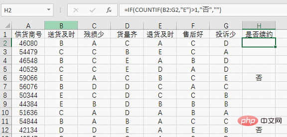
This time the range of COUNTIF changes OK, count the number of occurrences of "E" in the range B2:G2. Also pay attention to adding quotation marks. When the statistical result is greater than 1, it means that the supplier has more than two negative reviews (if you insist Use greater than or equal to 2, I have no objection), and then use IF to get the final result.
The last question I want to talk about must be familiar to partners in financial positions. Sometimes we will encounter this situation: There is a positive and a negative situation in a column of data. At this time, it is necessary to change the future The offset data is marked (extracted) , such as the example in the picture:
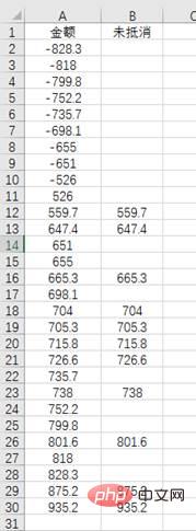
This problem may have caused headaches for many people. In fact, using Today's combination of these two functions is easy to solve. The formula is:
=IF(COUNTIF(A:A,-A2)=0,A2,"")
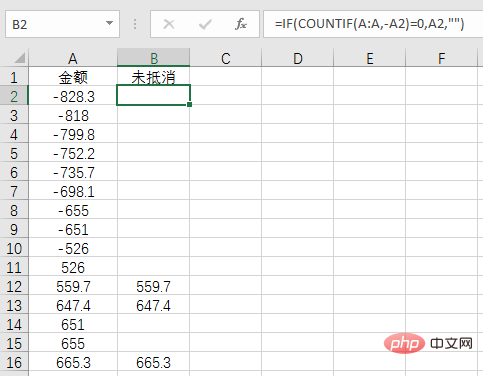
Pay attention to the condition -A2 in COUNTIF here, that is, find the number that can cancel each other out with A2. If not, get A2 through IF, and vice versa. Null value, using a negative sign cleverly solves a troublesome problem.
Through the above five cases, you may have a feeling that the combination of these two functions is relatively easier to understand than some other function combinations. As long as you find the right idea, this combination can be used for many problems. to handle. This is also true. If you are good at using COUNTIF to count various conditions, and then use the IF function to get more diverse results, ifcountif is often used to filter duplicate data. Solving problems does not necessarily require difficult functions. It is also very pleasant to use simple functions well.
Related learning recommendations: excel tutorial
The above is the detailed content of Excel function learning: Let's talk about how to use countif() (detailed case explanation). For more information, please follow other related articles on the PHP Chinese website!

Hot AI Tools

Undresser.AI Undress
AI-powered app for creating realistic nude photos

AI Clothes Remover
Online AI tool for removing clothes from photos.

Undress AI Tool
Undress images for free

Clothoff.io
AI clothes remover

AI Hentai Generator
Generate AI Hentai for free.

Hot Article
Hot Tools

Notepad++7.3.1
Easy-to-use and free code editor

SublimeText3 Chinese version
Chinese version, very easy to use

Zend Studio 13.0.1
Powerful PHP integrated development environment

Dreamweaver CS6
Visual web development tools

SublimeText3 Mac version
God-level code editing software (SublimeText3)
Hot Topics
 1371
1371
 52
52

 What should I do if the frame line disappears when printing in Excel?
Mar 21, 2024 am 09:50 AM
What should I do if the frame line disappears when printing in Excel?
Mar 21, 2024 am 09:50 AM
If when opening a file that needs to be printed, we will find that the table frame line has disappeared for some reason in the print preview. When encountering such a situation, we must deal with it in time. If this also appears in your print file If you have questions like this, then join the editor to learn the following course: What should I do if the frame line disappears when printing a table in Excel? 1. Open a file that needs to be printed, as shown in the figure below. 2. Select all required content areas, as shown in the figure below. 3. Right-click the mouse and select the "Format Cells" option, as shown in the figure below. 4. Click the “Border” option at the top of the window, as shown in the figure below. 5. Select the thin solid line pattern in the line style on the left, as shown in the figure below. 6. Select "Outer Border"
 How to filter more than 3 keywords at the same time in excel
Mar 21, 2024 pm 03:16 PM
How to filter more than 3 keywords at the same time in excel
Mar 21, 2024 pm 03:16 PM
Excel is often used to process data in daily office work, and it is often necessary to use the "filter" function. When we choose to perform "filtering" in Excel, we can only filter up to two conditions for the same column. So, do you know how to filter more than 3 keywords at the same time in Excel? Next, let me demonstrate it to you. The first method is to gradually add the conditions to the filter. If you want to filter out three qualifying details at the same time, you first need to filter out one of them step by step. At the beginning, you can first filter out employees with the surname "Wang" based on the conditions. Then click [OK], and then check [Add current selection to filter] in the filter results. The steps are as follows. Similarly, perform filtering separately again
 How to change excel table compatibility mode to normal mode
Mar 20, 2024 pm 08:01 PM
How to change excel table compatibility mode to normal mode
Mar 20, 2024 pm 08:01 PM
In our daily work and study, we copy Excel files from others, open them to add content or re-edit them, and then save them. Sometimes a compatibility check dialog box will appear, which is very troublesome. I don’t know Excel software. , can it be changed to normal mode? So below, the editor will bring you detailed steps to solve this problem, let us learn together. Finally, be sure to remember to save it. 1. Open a worksheet and display an additional compatibility mode in the name of the worksheet, as shown in the figure. 2. In this worksheet, after modifying the content and saving it, the dialog box of the compatibility checker always pops up. It is very troublesome to see this page, as shown in the figure. 3. Click the Office button, click Save As, and then
 How to type subscript in excel
Mar 20, 2024 am 11:31 AM
How to type subscript in excel
Mar 20, 2024 am 11:31 AM
eWe often use Excel to make some data tables and the like. Sometimes when entering parameter values, we need to superscript or subscript a certain number. For example, mathematical formulas are often used. So how do you type the subscript in Excel? ?Let’s take a look at the detailed steps: 1. Superscript method: 1. First, enter a3 (3 is superscript) in Excel. 2. Select the number "3", right-click and select "Format Cells". 3. Click "Superscript" and then "OK". 4. Look, the effect is like this. 2. Subscript method: 1. Similar to the superscript setting method, enter "ln310" (3 is the subscript) in the cell, select the number "3", right-click and select "Format Cells". 2. Check "Subscript" and click "OK"
 How to set superscript in excel
Mar 20, 2024 pm 04:30 PM
How to set superscript in excel
Mar 20, 2024 pm 04:30 PM
When processing data, sometimes we encounter data that contains various symbols such as multiples, temperatures, etc. Do you know how to set superscripts in Excel? When we use Excel to process data, if we do not set superscripts, it will make it more troublesome to enter a lot of our data. Today, the editor will bring you the specific setting method of excel superscript. 1. First, let us open the Microsoft Office Excel document on the desktop and select the text that needs to be modified into superscript, as shown in the figure. 2. Then, right-click and select the "Format Cells" option in the menu that appears after clicking, as shown in the figure. 3. Next, in the “Format Cells” dialog box that pops up automatically
 How to use the iif function in excel
Mar 20, 2024 pm 06:10 PM
How to use the iif function in excel
Mar 20, 2024 pm 06:10 PM
Most users use Excel to process table data. In fact, Excel also has a VBA program. Apart from experts, not many users have used this function. The iif function is often used when writing in VBA. It is actually the same as if The functions of the functions are similar. Let me introduce to you the usage of the iif function. There are iif functions in SQL statements and VBA code in Excel. The iif function is similar to the IF function in the excel worksheet. It performs true and false value judgment and returns different results based on the logically calculated true and false values. IF function usage is (condition, yes, no). IF statement and IIF function in VBA. The former IF statement is a control statement that can execute different statements according to conditions. The latter
 Where to set excel reading mode
Mar 21, 2024 am 08:40 AM
Where to set excel reading mode
Mar 21, 2024 am 08:40 AM
In the study of software, we are accustomed to using excel, not only because it is convenient, but also because it can meet a variety of formats needed in actual work, and excel is very flexible to use, and there is a mode that is convenient for reading. Today I brought For everyone: where to set the excel reading mode. 1. Turn on the computer, then open the Excel application and find the target data. 2. There are two ways to set the reading mode in Excel. The first one: In Excel, there are a large number of convenient processing methods distributed in the Excel layout. In the lower right corner of Excel, there is a shortcut to set the reading mode. Find the pattern of the cross mark and click it to enter the reading mode. There is a small three-dimensional mark on the right side of the cross mark.
 How to insert excel icons into PPT slides
Mar 26, 2024 pm 05:40 PM
How to insert excel icons into PPT slides
Mar 26, 2024 pm 05:40 PM
1. Open the PPT and turn the page to the page where you need to insert the excel icon. Click the Insert tab. 2. Click [Object]. 3. The following dialog box will pop up. 4. Click [Create from file] and click [Browse]. 5. Select the excel table to be inserted. 6. Click OK and the following page will pop up. 7. Check [Show as icon]. 8. Click OK.
