
 Topics
excel
Excel case sharing: How to use Excel to create an electronic inventory ledger? (Summary of inbound and outbound ledgers)
Topics
excel
Excel case sharing: How to use Excel to create an electronic inventory ledger? (Summary of inbound and outbound ledgers)
Excel case sharing: How to use Excel to create an electronic inventory ledger? (Summary of inbound and outbound ledgers)

Many warehouse managers have to summarize the inventory ledger balances every month. If they don’t know how to design the inventory ledger form, they have to work overtime every day. In fact, using three functions in excel, you can design the warehouse entry and exit in a few seconds. Ledger template solves the problem! Today, this article will share with you an article on how to use Excel to create an electronic inventory ledger. The author's explanation is from simple to deep, which is very helpful for beginners to learn. Come and take a look!

#Today I would like to share with you a case that a student encountered regarding the summary statistics of inventory ledger balances.
Briefly introduce this student’s problems and needs.
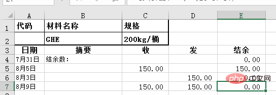
This trainee’s job is mainly to statistically manage the inventory accounts of various types of products. Now you need to summarize the balance quantities in the product inventory information tables of a large number of models into a worksheet.
As shown below:
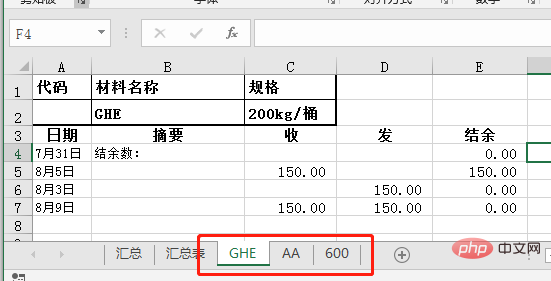
For example, GHE, AA, and 600 are three different models of products. The last line in column E is the latest balance of the product. Condition. (Note: The formats in each product model table are consistent)
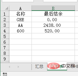
Now you need to use the product model as a row in the summary table to count the final balance of each product.
As shown in the figure below:
There are actually two problems when we want to achieve such a demand.
1. Reference the data in each product balance detail worksheet to the summary table.
2. How to return the final balance in the product model table.
Let’s take these two questions to solve the needs of this student.
1. Since references are used, we must be able to use the indirect function, whose main function is to return the reference specified by the text string.
Example:
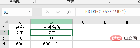
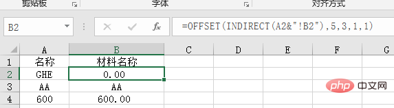
#A column is the name of the worksheet, by combining the text characters in cell A2 with !B2 merge builds a reference. I believe you must be familiar with cross-table matching in your daily work. The target cell references are composed of worksheet name, exclamation mark, and cell name , such as: GHE!B2.
Here we can directly return the contents of cell B2 in the GHE worksheet through the INDIRECT(A2&"!B2") function formula.
Let’s see if the content of cell B2 in the GHE worksheet is GHE.
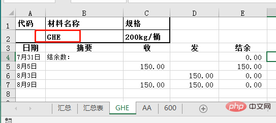
We see that the content of cell B2 in the GHE worksheet is indeed GHE.
2. The second question is how to return the final balance.
Taking the GHE worksheet as an example, our ultimate goal is to return the contents of cell E7 in the table, and it needs to follow the number of rows Change with change.
Seeing this, I believe many people will think of using the offset function to complete it
The function of the Offset function is to use the specified reference as the reference system and obtain a new reference through the given offset. The reference returned can be a cell or a range of cells. And you can specify the number of rows or columns to return. Reference serves as the reference region of the offset reference system. Reference must be a reference to a cell or a connected range of cells; otherwise, the OFFSET function returns the #VALUE! error value.
As shown below:
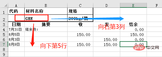
Function formula: =OFFSET(B2,5,3,1,1)
Meaning: Using B2 where the GHE worksheet is located as the reference cell, offset 3 columns to the right and 5 rows down to return the final balance of cell E7. 5 in the function formula means the fifth row, 3 means the third column, and the last two parameters are 1, which means only the content of one cell is returned.
Next we only need to nest the function formula with the indirect function formula in the first step:
=OFFSET(INDIRECT(A2&"!B2"), 5,3,1,1)
The static data return is done, so how can it change at any time as the number of rows changes?
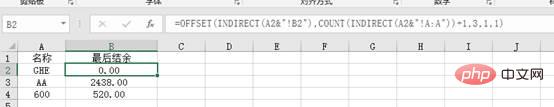
Because the date in column A in the table corresponds to the balance in column E, here we cleverly replace the number of rows with the count function, and use the count function to count the number of numerical cells in column A as the second parameter of OFFSET parameters. In this way, we can count the corresponding final balance data at any time as the number of rows changes.
The function formula is: COUNT(INDIRECT(A2&"!A:A")) 1, the reason for adding 1 is because there are only 4 cells in column A of the GHE worksheet that are numerical values , and in the previous case we needed to shift downward by 5 lines, so we need to add 1 to this.
Final function formula:
=OFFSET(INDIRECT(A2&"!B2"),COUNT(INDIRECT(A2&"!A:A")) 1,3,1, 1)
Let’s briefly summarize and sort out:
The main difficulty in this case is how to reference the last row of values in the specified column, here We used the offset and indirect functions to complete the reference of the specified data, and at the same time completed the dynamic update and search of the specified cells through the count function. Finally, it is possible to quickly count product names and return the final balance of the corresponding inventory ledger.
Related learning recommendations: excel tutorial
The above is the detailed content of Excel case sharing: How to use Excel to create an electronic inventory ledger? (Summary of inbound and outbound ledgers). For more information, please follow other related articles on the PHP Chinese website!

Hot AI Tools

Undresser.AI Undress
AI-powered app for creating realistic nude photos

AI Clothes Remover
Online AI tool for removing clothes from photos.

Undress AI Tool
Undress images for free

Clothoff.io
AI clothes remover

AI Hentai Generator
Generate AI Hentai for free.

Hot Article
Hot Tools

Notepad++7.3.1
Easy-to-use and free code editor

SublimeText3 Chinese version
Chinese version, very easy to use

Zend Studio 13.0.1
Powerful PHP integrated development environment

Dreamweaver CS6
Visual web development tools

SublimeText3 Mac version
God-level code editing software (SublimeText3)
Hot Topics
 1377
1377
 52
52

 What should I do if the frame line disappears when printing in Excel?
Mar 21, 2024 am 09:50 AM
What should I do if the frame line disappears when printing in Excel?
Mar 21, 2024 am 09:50 AM
If when opening a file that needs to be printed, we will find that the table frame line has disappeared for some reason in the print preview. When encountering such a situation, we must deal with it in time. If this also appears in your print file If you have questions like this, then join the editor to learn the following course: What should I do if the frame line disappears when printing a table in Excel? 1. Open a file that needs to be printed, as shown in the figure below. 2. Select all required content areas, as shown in the figure below. 3. Right-click the mouse and select the "Format Cells" option, as shown in the figure below. 4. Click the “Border” option at the top of the window, as shown in the figure below. 5. Select the thin solid line pattern in the line style on the left, as shown in the figure below. 6. Select "Outer Border"
 How to filter more than 3 keywords at the same time in excel
Mar 21, 2024 pm 03:16 PM
How to filter more than 3 keywords at the same time in excel
Mar 21, 2024 pm 03:16 PM
Excel is often used to process data in daily office work, and it is often necessary to use the "filter" function. When we choose to perform "filtering" in Excel, we can only filter up to two conditions for the same column. So, do you know how to filter more than 3 keywords at the same time in Excel? Next, let me demonstrate it to you. The first method is to gradually add the conditions to the filter. If you want to filter out three qualifying details at the same time, you first need to filter out one of them step by step. At the beginning, you can first filter out employees with the surname "Wang" based on the conditions. Then click [OK], and then check [Add current selection to filter] in the filter results. The steps are as follows. Similarly, perform filtering separately again
 How to change excel table compatibility mode to normal mode
Mar 20, 2024 pm 08:01 PM
How to change excel table compatibility mode to normal mode
Mar 20, 2024 pm 08:01 PM
In our daily work and study, we copy Excel files from others, open them to add content or re-edit them, and then save them. Sometimes a compatibility check dialog box will appear, which is very troublesome. I don’t know Excel software. , can it be changed to normal mode? So below, the editor will bring you detailed steps to solve this problem, let us learn together. Finally, be sure to remember to save it. 1. Open a worksheet and display an additional compatibility mode in the name of the worksheet, as shown in the figure. 2. In this worksheet, after modifying the content and saving it, the dialog box of the compatibility checker always pops up. It is very troublesome to see this page, as shown in the figure. 3. Click the Office button, click Save As, and then
 How to type subscript in excel
Mar 20, 2024 am 11:31 AM
How to type subscript in excel
Mar 20, 2024 am 11:31 AM
eWe often use Excel to make some data tables and the like. Sometimes when entering parameter values, we need to superscript or subscript a certain number. For example, mathematical formulas are often used. So how do you type the subscript in Excel? ?Let’s take a look at the detailed steps: 1. Superscript method: 1. First, enter a3 (3 is superscript) in Excel. 2. Select the number "3", right-click and select "Format Cells". 3. Click "Superscript" and then "OK". 4. Look, the effect is like this. 2. Subscript method: 1. Similar to the superscript setting method, enter "ln310" (3 is the subscript) in the cell, select the number "3", right-click and select "Format Cells". 2. Check "Subscript" and click "OK"
 How to set superscript in excel
Mar 20, 2024 pm 04:30 PM
How to set superscript in excel
Mar 20, 2024 pm 04:30 PM
When processing data, sometimes we encounter data that contains various symbols such as multiples, temperatures, etc. Do you know how to set superscripts in Excel? When we use Excel to process data, if we do not set superscripts, it will make it more troublesome to enter a lot of our data. Today, the editor will bring you the specific setting method of excel superscript. 1. First, let us open the Microsoft Office Excel document on the desktop and select the text that needs to be modified into superscript, as shown in the figure. 2. Then, right-click and select the "Format Cells" option in the menu that appears after clicking, as shown in the figure. 3. Next, in the “Format Cells” dialog box that pops up automatically
 How to use the iif function in excel
Mar 20, 2024 pm 06:10 PM
How to use the iif function in excel
Mar 20, 2024 pm 06:10 PM
Most users use Excel to process table data. In fact, Excel also has a VBA program. Apart from experts, not many users have used this function. The iif function is often used when writing in VBA. It is actually the same as if The functions of the functions are similar. Let me introduce to you the usage of the iif function. There are iif functions in SQL statements and VBA code in Excel. The iif function is similar to the IF function in the excel worksheet. It performs true and false value judgment and returns different results based on the logically calculated true and false values. IF function usage is (condition, yes, no). IF statement and IIF function in VBA. The former IF statement is a control statement that can execute different statements according to conditions. The latter
 Where to set excel reading mode
Mar 21, 2024 am 08:40 AM
Where to set excel reading mode
Mar 21, 2024 am 08:40 AM
In the study of software, we are accustomed to using excel, not only because it is convenient, but also because it can meet a variety of formats needed in actual work, and excel is very flexible to use, and there is a mode that is convenient for reading. Today I brought For everyone: where to set the excel reading mode. 1. Turn on the computer, then open the Excel application and find the target data. 2. There are two ways to set the reading mode in Excel. The first one: In Excel, there are a large number of convenient processing methods distributed in the Excel layout. In the lower right corner of Excel, there is a shortcut to set the reading mode. Find the pattern of the cross mark and click it to enter the reading mode. There is a small three-dimensional mark on the right side of the cross mark.
 How to insert excel icons into PPT slides
Mar 26, 2024 pm 05:40 PM
How to insert excel icons into PPT slides
Mar 26, 2024 pm 05:40 PM
1. Open the PPT and turn the page to the page where you need to insert the excel icon. Click the Insert tab. 2. Click [Object]. 3. The following dialog box will pop up. 4. Click [Create from file] and click [Browse]. 5. Select the excel table to be inserted. 6. Click OK and the following page will pop up. 7. Check [Show as icon]. 8. Click OK.
