Excel function learning: Let's talk about N()--a function that converts to a numerical value

The function I brought to you today is very simple. It has only one letter, which is N!

The function of the N function is to convert non-numeric content in Excel into numerical values, such as converting dates into serial values, TRUE into 1, FALSE into 0, text content into 0, etc. It needs to be emphasized. The next thing is that the N function cannot convert error values.

Okay, I’ve finished talking about the functions of the ExcelN function. I didn’t realize how powerful it is. The usefulness of the function seems to be limited.

Whether this is the case, let us illustrate it through some examples. After reading the examples, if you feel that the N function is really powerful, be sure to leave a message in the comment area~~~

1. Application of N function in simplifying formulas

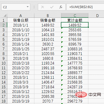
Example 1: We usually use sum directly to calculate the cumulative amount, enter the formula =SUM($B$2) in cell C2 :B2), double-click to fill down to get the cumulative amount.

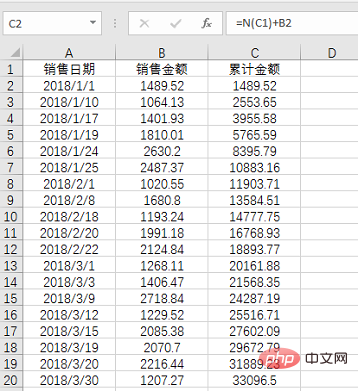
In fact, you can use the N function to change the C2 cell formula to: =B2 N(C1), double-click to fill, and you can get the daily cumulative total amount.

This example does not show the power of the N function, just think of it as a warm-up for the N function!

What, I can’t understand the second formula!

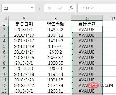
N is to convert the text into 0. We do not need the title C1 when calculating the total. Without this conversion, errors will occur and the text cannot be calculated directly.

Let’s look at the second example. This time the N function is about to show its power!

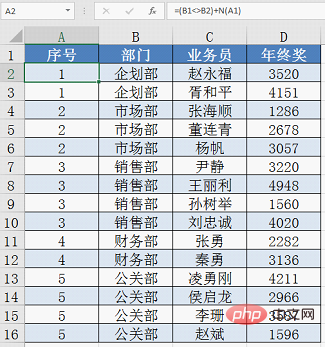
Example 2: If there are different departments, the serial number will be increased by 1;

Enter the traditional formula in cell A2: =SUMPRODUCT(1/COUNTIF(B$2:B2,B$2 :B2))

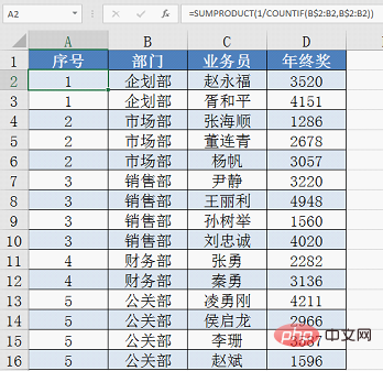
After using the N function, the formula in cell A2 becomes: =(B1B2) N (A1)

Don’t you understand? Do you still think the N function is simple or useless?

Formula analysis:

First determine whether B1 and B2 are equal. If not, it is TRUE, which is 1, plus the value of N (A1) 0, So the result of cell A2 is 1. In the drop-down formula, B2 and B3 are equal, the result is FALSE, which is 0, plus the value of N (A2) is 1, so the result of cell A3 is 1. And so on.

The second example only shows the advantages of the N function in simplifying formulas. As everyone knows more and more about the application of formula functions, they will understand this.

2. Application of N function in conditional statistics

Example 3: Conditional counting

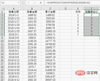
This kind of problem cannot be calculated using COUNTIF, because the conditional range of COUNTIF can only be referenced using cell ranges and cannot be obtained using functions. There is no ready-made month in the data source. It must be processed through the MONTH function.

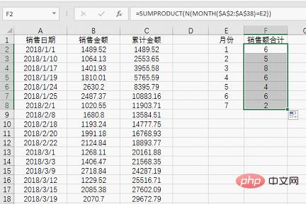
The SUMPRODUCT function is usually used for statistics, but the statistical result is 0. The reason is that SUMPRODUCT cannot directly count logical values. At this time, the N function is needed:

Example 4: Example of matching with IF function

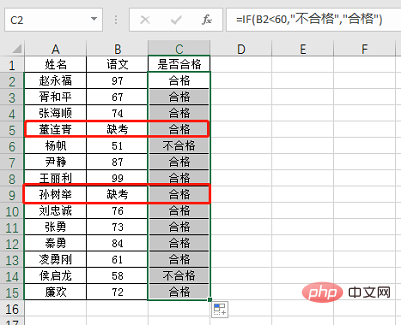
This example is very simple. If your score is less than 60 points, you will be unqualified. If you miss the exam, you will be considered unqualified.

When only one if is used, there will be wrong results. At this time, you can use the N function:

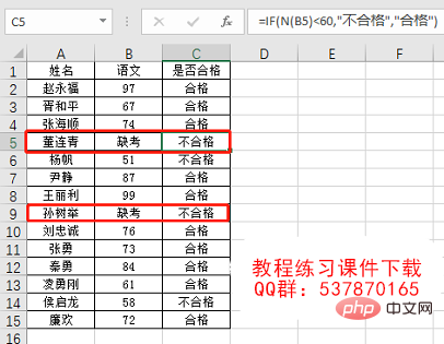
Principle Just use the N function to convert the text to 0 and then compare.

The above content is relatively easy to understand. You can see that the N function has many uses. The next content is more advanced, and it is time for the N function to show its true strength. If you don’t believe it, take a look:

3. The fantasy combination of VLOOKUP N

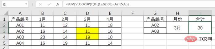
The example is as shown below: Please specify multiple products in a certain Total monthly sales

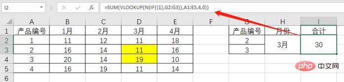
Normally, multi-condition summation problems are usually solved using SUMPRODUCT, but with the intervention of the N function, This problem was solved by the most well-known VLOOKUP (of course, SUM also takes credit).

In this formula: =SUM(VLOOKUP(N(IF({1},G2:G3)),A2:E5,4,))

VLOOKUP was naturally written like this at the beginning: =SUM(VLOOKUP(G2:G3,A2:E5,4,))

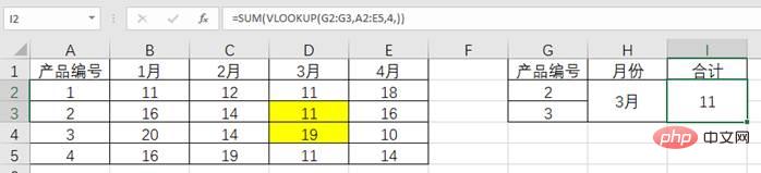
The first parameter is two, so two results are also obtained. After summing, it is found that only the first data does not achieve the purpose of summing, but it is written as N(IF({1}, G2:G3) is fine. This is a magical combination. The first parameter of IF is 1, which is TRUE, so if the second parameter of IF is returned, G2:G3, and then processed by the N function, the VLOOKUP reference can be made. Got multiple results.

What is the principle?

I can’t explain it clearly, so I say it is a fantasy combination... Remember this routine and just copy it when you need to use it.

Some friends may ask if the product number is not a number, such as this, there will be a problem:

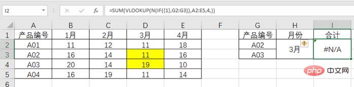
I think this is the case You can answer, because the N function is only valid for numbers. Such numbers are obviously text. At this time, you need to replace N with T:

Okay Now, it’s almost time for the N function to take a rest. I guess many friends have almost fainted because the formula is too difficult to understand...

The last example, let N add a comment to our formula Explanation, I believe not many people know how to use this.

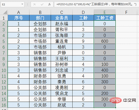
4. N function adds instructions to your formula

The following figure is an example : Determine seniority wages based on seniority. The rule is very simple. If the seniority exceeds 3 years, it will increase by 100 every year. Generally, we use the formula =IF(D2>3,(D2-3)*100,0) to achieve the purpose. However, in order to make the calculation method more clear to people looking at the table, you can use the N function to write a literal description in the formula, as shown in the edit bar below. The formula is clear and does not affect the result.

Note: When the formula result is a number, use the N() method. When the formula result is text, use the &T() method. Of course, it can also be used here. Use comments to add explanations, but does this method seem more mysterious?

Simple functions are often not simple, and the road to functions is still long. Let us accompany you along the way to explore more interesting and practical skills!

Related learning recommendations: excel tutorial

The above is the detailed content of Excel function learning: Let's talk about N()--a function that converts to a numerical value. For more information, please follow other related articles on the PHP Chinese website!