Practical Excel skills sharing: Use Power Query to merge workbooks in folders

I previously introduced you to the use of EXCEL’s new function Power Query to summarize the worksheets in the workbook, but the function of Power Query is far more than that. Today I will introduce it to you. More advanced merging techniques: Use Power Query to merge workbooks in folders.

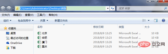
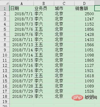
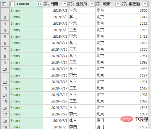
As shown below, there are sales data for four regions in the "Sales" folder on the desktop. The title names in each workbook are consistent, and the order can be different. The value of the city column in each workbook is the name of the workbook, which is convenient for viewing the merge effect later.

#The operation is as follows:

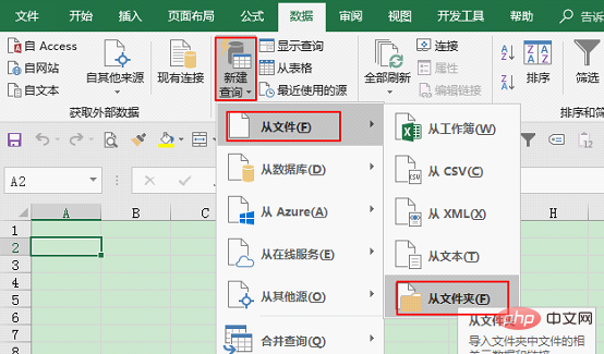
Close the files in the folder, create a new workbook, click on the Data tab, [Get and Transform] group "New Query" --- "From File" --- "From Folder".

Enter the folder path, or browse to select the folder location and click OK.

This interface lists all the workbooks in the folder, click Edit.

Entered the Power Query editor interface. The top is the menu bar, the middle is the table area and the data that will be returned to the worksheet at the end. The query setting window on the right displays the Power Query operation record.

As introduced before, the green font in the "Content" column means that this cell contains a file. Click on a cell to preview its contents. (

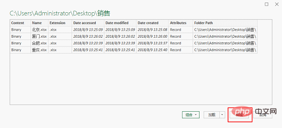
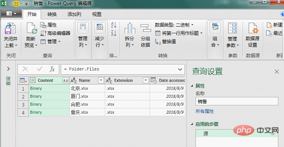
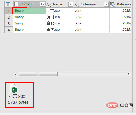
Note: When previewing the content in the cell, you should place the mouse on the blank space in the cell, not on the text. Clicking on the text will directly open the file in the cell) Since the file is directly opened from the folder The extracted files are all in binary format, so the workbook in binary format appears in the preview pane below.

Binary as a binary file cannot be displayed in the table, so what we have to do is to change it into table format and then expand the data into the table inside. Delete other unnecessary columns first.

Select the "Content" column, click "Delete Column" - "Delete Other Columns" in the [Manage Columns] group under the Home tab.

In this way, all other columns except the "Content" column are deleted.

#So how to convert the binary file into an ordinary table requires the use of Power Query's special programming language-M language. Here I will introduce you to a commonly used function.

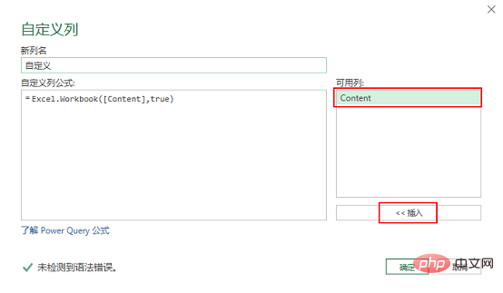
Click "Custom Column" in the [General] group under the Add Column option.

In the Custom Column window, enter =Excel.Workbook([Content],true) in the "Custom Column Formula", where "[ Content]" You can click "Content" in the available column on the right, and then click on the lower right corner to insert (Note: the capitalization of the formula must not be wrong).

Formula analysis:

Excel.Workbook

Function: Return the records of the worksheet from the Excel workbook.

Parameters: Excel.Workbook(workbook as binary, optional useHeaders as nullable logical, optionaldelayTypes as nullable logical) as table

This function returns a table. The first parameter workbook is in binary format, and the second parameter is the logical value of the optional parameter. true means using the title of the original table as the new table. The title, the default is false, means replacing the title of the original worksheet with the new column name. Don't worry about the third parameter.

Here we still use the original title of the form, so fill in true. This saves the subsequent step of improving the first line of the title.

The new column is added successfully. Preview one of the cells. What is shown below is a table-style workbook. This can be directly extended to the table.

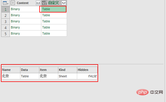
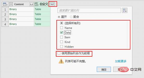
The "Data" column displays a table in Table format, including the data in the table. Here we only need to extract this column. . Click the expand button in the upper right corner of the custom column, select the expanded column "Data", and uncheck "Use original column name as prefix".

The column name becomes "Data". At this time, we preview the data in "Data", and what appears below is the original data in the table. Then extract all the data below.

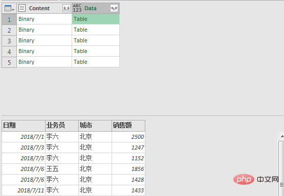
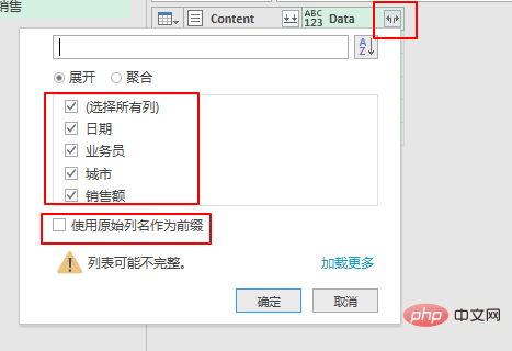
Similarly click the expand button on the upper right side of the custom column, select expand all columns, and do not check "Use original column name as prefix".

In this way, we obtain the data in the worksheet by drilling layer by layer.

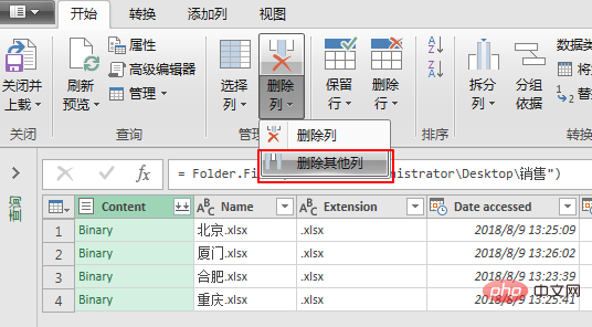
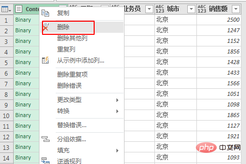
Finally delete the "Content" column. Select the "Content" column and right-click to delete it.

#Finally, just upload this table to the form.

Click "Close and Upload" in the [Close] group under the Home tab.

#The data will be summarized in the worksheet.

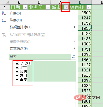
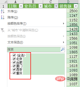
When you click the filter button in the "City" column, you will see that the data in the four workbooks are all in the table.

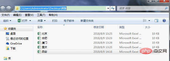
What happens when there is one more workbook in the folder? Try placing a new workbook "Xi'an" in this folder.

Go back to the table where you just made statistics, click [ under the data tab "Refresh All" in the Connection] group.

The city column has "Xi'an" added, which represents the data of this new workbook was added.

Summary: Power Query merges folders. As long as the titles in each worksheet are the same, it can be merged and summarized. This method does not care about the folders. Any number of workbooks can be merged. And any data changes can be updated with one click through all refresh.

Power Query is a powerful tool for EXCEL data analysis. Through simple graphical operations, combined with its own M language and through the operation recorder, it helps us to operate more data in a unified manner and quickly complete data processing and optimization. Moreover, it is faster to get started and easier to operate than VBA, and graphical operation can meet most of our needs. Everyone, hurry up and learn!

Related learning recommendations: excel tutorial

The above is the detailed content of Practical Excel skills sharing: Use Power Query to merge workbooks in folders. For more information, please follow other related articles on the PHP Chinese website!