
 Topics
excel
An in-depth analysis of the Excel Tiger Balm screening formula 'INDEX-SMALL-IF-ROW'
Topics
excel
An in-depth analysis of the Excel Tiger Balm screening formula 'INDEX-SMALL-IF-ROW'
An in-depth analysis of the Excel Tiger Balm screening formula 'INDEX-SMALL-IF-ROW'

This article shares how Excel uses formula filtering to complete one-to-many search. It is a classic excel filtering function formula to automatically find formula data.

I always hear experts say that there is a Tiger Balm formula, but what exactly is the Tiger Balm formula, and what can this Excel formula do? Let’s take a look at the following rendering first:
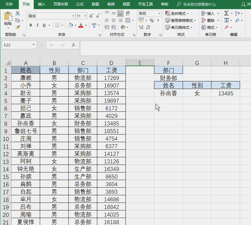
This example is a typical one-to-many search. The search condition is department, and each department corresponds to it in the data source. All are multiple data, and the main purpose of the Tiger Balm formula is to solve some relatively complex problems such as one-to-many search. The formula in the animation above is:
=IFERROR(INDEX($A$2:$D$21,SMALL(IF($C$2:$C$21=$F$2,ROW($1:$20 ),99),ROW(A1)),MATCH(F$3,$A$1:$D$1,0)),"")
Perhaps many friends will be amazed when they see this formula : I can’t understand such a long formula!
Today I will work with you to crack this incomprehensible but very powerful formula routine. Please be patient and read on...
The above formula uses a total of six functions: IFERROR, INDEX , SMALL, IF, ROW and MATCH, of which IFERROR and MATCH are the two auxiliary functions in this example, and the remaining four INDEX-SMALL-IF-ROW are the snake oil formula.
So let’s learn the principle of this core part first:
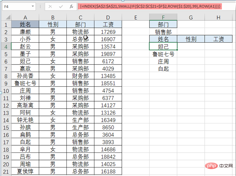
The formula of cell F4 is:
=INDEX($A$2:$A$21, SMALL(IF($C$2:$C$21=$F$2,ROW($1:$20),99),ROW(A1)))
Let’s start with INDEX. The basic function of this function is to give an area, and then return the search result according to the corresponding row and column position. In the above figure, the data area searched by INDEX is the area $A$2:$A$21 where the name is located.
The basic structure of the INDEX function is: INDEX (search area, row and column). If the area is a single row or column, one of the last two parameters can be omitted. In layman's terms, when you take a movie ticket to find a seat, the seats in the entire hall are the area, and the rows and seats are the last two parameters in the formula. In this way, the target location can be found accurately.
In the above example, the area is in one column, so we only need to determine which row each data is in.
Understanding this, our focus should be on the second parameter of INDEX:
SMALL(IF($C$2:$C$21=$F$2 ,ROW($1:$20),99),ROW(A1))
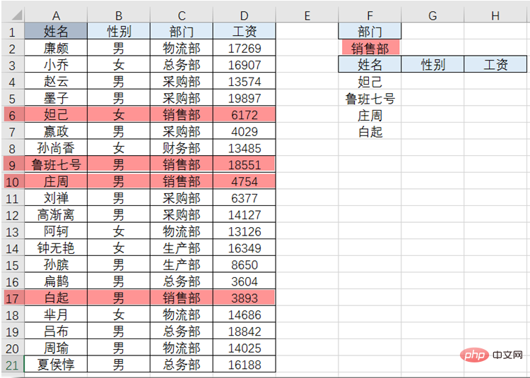
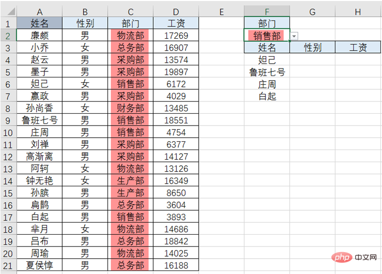
Pay attention to the picture above, the sales department has a total Four records, respectively in rows 5, 8, 9 and 16 of the data area (the data area starts from the second row).
So we hope that when the formula is pulled down, the second parameter of INDEX is the four numbers 5, 8, 9 and 16 (this must be understood).
Attention, we are about to come into contact with the core part of Tiger Balm, please maintain a high degree of concentration...
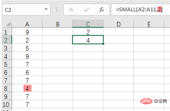
The basic structure of the SMALL function: SMALL (a set of numbers, The smallest number)
It is recommended that you simulate a simple data to fully understand this function. The method is as follows:
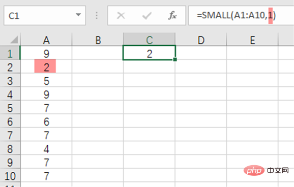
In Enter some numbers in column A. The formula means the smallest number in this column. The result is 2. It’s easy to understand, right? Change the second parameter of the formula to 2 and look at the result:
The penultimate one is 4.
If you want to continue to get the third smallest number, I think everyone can think of what to do, but there will be a problem. We can only modify the second parameter manually and cannot achieve this parameter through drop-down. Change, if you want to be able to pull down, the second parameter needs to use the ROW function, which is modified like this:
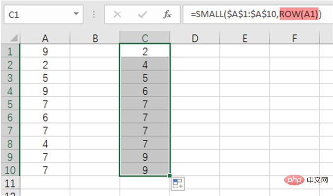
ROW function is very simple, what you get is The row number of the parameter. Through this formula, we can sort the data in column A from small to large. Do you think it is interesting?
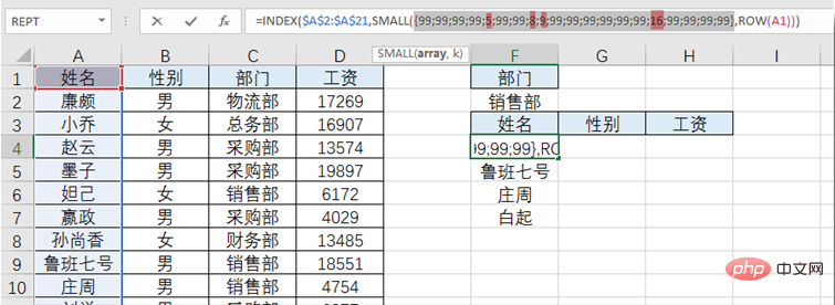
Back to our Tiger Balm formula, remember what the four numbers 5, 8, 9 and 16 mean. We need to use the SMALL function to get these four numbers in sequence. The idea is to determine whether column C is Consistent with F2, if the line number is the same, if it is different, a number larger than the maximum line number is obtained (the purpose is to prevent it from being found):
To achieve this goal, the intervention of the IF function is needed, so there is:
IF($C$2:$C$21=$F$2,ROW($1:$20),99), use this paragraph as the first parameter of SMALL.
Regarding this IF, it is easier to understand. We can use F9 to see the results of this formula:
Because we There are only 20 pieces of data, so it is enough to use 99 as the third parameter of IF. If the amount of data is relatively large, you can use 9^9, which means 9 raised to the 9th power. Anyway, it is large enough.
If you understand this IF, look at this paragraph againSMALL(IF($C$2:$C$21=$F$2,ROW($1:$20),99),ROW(A1)) Isn’t it so dizzy?
Regarding the SMALL part, you must understand that when the formula is pulled down, we get the numbers we want to get one by one, and then use these numbers as the second parameter of INDEX to get what we ultimately need. result.
The core of Tiger Balm is INDEX, SMALL, IF and ROW. Please be sure to think about it again and again to understand this part of the principle. There is another very important point that needs to be emphasized. The tiger balm formula is an array formula, so we need to hold down Ctrl and shift and press Enter.
As for the initial formula, considering that we need to find the contents of multiple columns, the data area of INDEX uses $A$2:$D$21. When there are multiple columns, you need to provide the column position to find the target value. , so use MATCH(F$3,$A$1:$D$1,0) to determine which column the data is in.
The data of each department is different. We need to pull down the formula a few more lines. At this time, some error values will be generated. Use the IFERROR function in the outermost layer of the formula to mask the error values, so that The query results look very clean.
Today I just used an example of one-to-many search to explain the principle of the Tiger Balm formula. In fact, there are many formulas for Tiger Balm. If you like it, continue to share related examples in the future. Of course, if you finish reading this article It would be even better if you can interpret some complex formulas yourself.
Related learning recommendations: excel tutorial
The above is the detailed content of An in-depth analysis of the Excel Tiger Balm screening formula 'INDEX-SMALL-IF-ROW'. For more information, please follow other related articles on the PHP Chinese website!

Hot AI Tools

Undresser.AI Undress
AI-powered app for creating realistic nude photos

AI Clothes Remover
Online AI tool for removing clothes from photos.

Undress AI Tool
Undress images for free

Clothoff.io
AI clothes remover

Video Face Swap
Swap faces in any video effortlessly with our completely free AI face swap tool!

Hot Article
Hot Tools

Notepad++7.3.1
Easy-to-use and free code editor

SublimeText3 Chinese version
Chinese version, very easy to use

Zend Studio 13.0.1
Powerful PHP integrated development environment

Dreamweaver CS6
Visual web development tools

SublimeText3 Mac version
God-level code editing software (SublimeText3)
Hot Topics
 1386
1386
 52
52

 What should I do if the frame line disappears when printing in Excel?
Mar 21, 2024 am 09:50 AM
What should I do if the frame line disappears when printing in Excel?
Mar 21, 2024 am 09:50 AM
If when opening a file that needs to be printed, we will find that the table frame line has disappeared for some reason in the print preview. When encountering such a situation, we must deal with it in time. If this also appears in your print file If you have questions like this, then join the editor to learn the following course: What should I do if the frame line disappears when printing a table in Excel? 1. Open a file that needs to be printed, as shown in the figure below. 2. Select all required content areas, as shown in the figure below. 3. Right-click the mouse and select the "Format Cells" option, as shown in the figure below. 4. Click the “Border” option at the top of the window, as shown in the figure below. 5. Select the thin solid line pattern in the line style on the left, as shown in the figure below. 6. Select "Outer Border"
 How to filter more than 3 keywords at the same time in excel
Mar 21, 2024 pm 03:16 PM
How to filter more than 3 keywords at the same time in excel
Mar 21, 2024 pm 03:16 PM
Excel is often used to process data in daily office work, and it is often necessary to use the "filter" function. When we choose to perform "filtering" in Excel, we can only filter up to two conditions for the same column. So, do you know how to filter more than 3 keywords at the same time in Excel? Next, let me demonstrate it to you. The first method is to gradually add the conditions to the filter. If you want to filter out three qualifying details at the same time, you first need to filter out one of them step by step. At the beginning, you can first filter out employees with the surname "Wang" based on the conditions. Then click [OK], and then check [Add current selection to filter] in the filter results. The steps are as follows. Similarly, perform filtering separately again
 How to change excel table compatibility mode to normal mode
Mar 20, 2024 pm 08:01 PM
How to change excel table compatibility mode to normal mode
Mar 20, 2024 pm 08:01 PM
In our daily work and study, we copy Excel files from others, open them to add content or re-edit them, and then save them. Sometimes a compatibility check dialog box will appear, which is very troublesome. I don’t know Excel software. , can it be changed to normal mode? So below, the editor will bring you detailed steps to solve this problem, let us learn together. Finally, be sure to remember to save it. 1. Open a worksheet and display an additional compatibility mode in the name of the worksheet, as shown in the figure. 2. In this worksheet, after modifying the content and saving it, the dialog box of the compatibility checker always pops up. It is very troublesome to see this page, as shown in the figure. 3. Click the Office button, click Save As, and then
 How to type subscript in excel
Mar 20, 2024 am 11:31 AM
How to type subscript in excel
Mar 20, 2024 am 11:31 AM
eWe often use Excel to make some data tables and the like. Sometimes when entering parameter values, we need to superscript or subscript a certain number. For example, mathematical formulas are often used. So how do you type the subscript in Excel? ?Let’s take a look at the detailed steps: 1. Superscript method: 1. First, enter a3 (3 is superscript) in Excel. 2. Select the number "3", right-click and select "Format Cells". 3. Click "Superscript" and then "OK". 4. Look, the effect is like this. 2. Subscript method: 1. Similar to the superscript setting method, enter "ln310" (3 is the subscript) in the cell, select the number "3", right-click and select "Format Cells". 2. Check "Subscript" and click "OK"
 How to set superscript in excel
Mar 20, 2024 pm 04:30 PM
How to set superscript in excel
Mar 20, 2024 pm 04:30 PM
When processing data, sometimes we encounter data that contains various symbols such as multiples, temperatures, etc. Do you know how to set superscripts in Excel? When we use Excel to process data, if we do not set superscripts, it will make it more troublesome to enter a lot of our data. Today, the editor will bring you the specific setting method of excel superscript. 1. First, let us open the Microsoft Office Excel document on the desktop and select the text that needs to be modified into superscript, as shown in the figure. 2. Then, right-click and select the "Format Cells" option in the menu that appears after clicking, as shown in the figure. 3. Next, in the “Format Cells” dialog box that pops up automatically
 How to use the iif function in excel
Mar 20, 2024 pm 06:10 PM
How to use the iif function in excel
Mar 20, 2024 pm 06:10 PM
Most users use Excel to process table data. In fact, Excel also has a VBA program. Apart from experts, not many users have used this function. The iif function is often used when writing in VBA. It is actually the same as if The functions of the functions are similar. Let me introduce to you the usage of the iif function. There are iif functions in SQL statements and VBA code in Excel. The iif function is similar to the IF function in the excel worksheet. It performs true and false value judgment and returns different results based on the logically calculated true and false values. IF function usage is (condition, yes, no). IF statement and IIF function in VBA. The former IF statement is a control statement that can execute different statements according to conditions. The latter
 Where to set excel reading mode
Mar 21, 2024 am 08:40 AM
Where to set excel reading mode
Mar 21, 2024 am 08:40 AM
In the study of software, we are accustomed to using excel, not only because it is convenient, but also because it can meet a variety of formats needed in actual work, and excel is very flexible to use, and there is a mode that is convenient for reading. Today I brought For everyone: where to set the excel reading mode. 1. Turn on the computer, then open the Excel application and find the target data. 2. There are two ways to set the reading mode in Excel. The first one: In Excel, there are a large number of convenient processing methods distributed in the Excel layout. In the lower right corner of Excel, there is a shortcut to set the reading mode. Find the pattern of the cross mark and click it to enter the reading mode. There is a small three-dimensional mark on the right side of the cross mark.
 How to insert excel icons into PPT slides
Mar 26, 2024 pm 05:40 PM
How to insert excel icons into PPT slides
Mar 26, 2024 pm 05:40 PM
1. Open the PPT and turn the page to the page where you need to insert the excel icon. Click the Insert tab. 2. Click [Object]. 3. The following dialog box will pop up. 4. Click [Create from file] and click [Browse]. 5. Select the excel table to be inserted. 6. Click OK and the following page will pop up. 7. Check [Show as icon]. 8. Click OK.
