

Practical Excel skills sharing: 5 shortcut keys to improve work efficiency

This article will share with you the 5 most commonly used Excel shortcut keys to improve work efficiency, so that you can become a master in the eyes of your boss who can use the keyboard to make tables without the mouse. I hope it will be helpful to everyone.

#Everyone can use Excel, with varying levels of skill. If you can open this article today, you must want to improve your Excel skills. As the saying goes, only after you have high standards can you improve. So today I plan to follow the investment banking standards - throw away the mouse and just use the keyboard to share with you some of the most commonly used Excel shortcut keys.
The most commonly used shortcut keys in Excel 1: Ctrl arrows (up, down, left, and right)
If there is content in each row of the table, this operation can Allows you to jump from the "top" to the "bottom" of the table area with one click.
[Case]
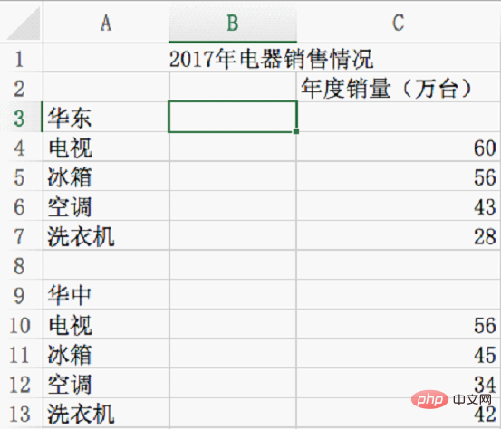
We usually deal with a large series of data, such as the annual employee performance table, etc. There are hundreds of rows of data, and we can't rub the mouse. Scroll wheel or keep pressing the down arrow. 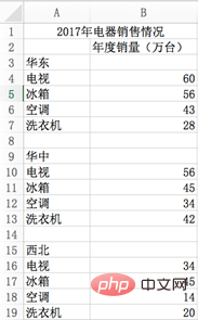
For example, if you want to jump from East China to Central China, first select the cell in East China, then hold down the Ctrl down arrow, and it will jump directly to cell A7, and then press the arrow again to jump to Cell A9;
If you want to select these at the same time, you have to hold down the Shift Ctrl down arrow.
【Summary】
Ctrl arrow can jump quickly. If there is an empty row in the middle, jump to the previous row of the empty row. Ctlr shift up/down arrows can quickly select consecutive multi-line areas.
The most commonly used Excel shortcut key 2: Shift Space
This function can quickly select an entire row of data.
For example, if your boss is discussing with you the sales of electrical appliances last year, you can select the fourth row of TV sales in East China at once, and visually distinguish them clearly without moving the mouse. The boss must look at you differently.
[Case]
I now want to turn all the text on the sales situation in East China into red. Without using the mouse, first hold down Shift + Space to select line 3, then release. Then hold down Shift ↓ and select lines 3 to 7 in sequence, and then change their font color to red.
【Summary】
Shift space can quickly select an entire line; hold down the Shift key and click multiple times The up/down arrow can select multiple rows continuously. The two methods can be used together to quickly select many rows continuously.
The 3 most commonly used shortcut keys in Excel: Ctrl D (copy top to bottom) and Ctrl R (copy left to right)
Very Commonly used functions, Ctrl D is to copy the content above to the bottom, D means down; Ctrl R is to copy the content on the left to the right, R means right.
[Case]
As shown below, cell B3 has no content. Press Ctrl R to copy the content of A3; then hold down Shift and press down arrow, select B3:B7, and press Ctrl D to copy all the contents of B3.
##[Summary]
Ctrl D/R is very important for daily work Commonly used functions. With this pair of shortcut keys, there's no need to copy and then paste.The most commonly used shortcut keys in Excel 4: F2 to edit cell content
If you need to modify the cell content, just press F2 Call up the cursor. When only a cell is selected, inputting content directly will replace the original content. And use F2 to add content based on the original.
The most commonly used Excel shortcut keys 5: Alt Enter (line break within each)
This function requires holding down F2 first to enter the state of editing cell content, then press the left and right arrow keys to move the cursor to the corresponding position, and press Alt Enter to force a new line.[Case]
As shown below, the number of words in A7 exceeds the cell size. It needs to be changed to two lines. The operation process is as follows: animation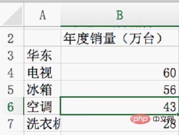
Have you got all the above shortcut keys? Although you don’t need to force yourself to give up the mouse and use the keyboard when you usually work, when your boss or colleague encounters a problem and is puzzled, you go over and just click the keyboard to solve it, and you are instantly in their mind. So tall! Those who can get promotions and salary increases, don’t they do things that their bosses can’t do~
Related learning recommendations: excel tutorial
The above is the detailed content of Practical Excel skills sharing: 5 shortcut keys to improve work efficiency. For more information, please follow other related articles on the PHP Chinese website!

Hot AI Tools

Undresser.AI Undress
AI-powered app for creating realistic nude photos

AI Clothes Remover
Online AI tool for removing clothes from photos.

Undress AI Tool
Undress images for free

Clothoff.io
AI clothes remover

AI Hentai Generator
Generate AI Hentai for free.

Hot Article
Hot Tools

Notepad++7.3.1
Easy-to-use and free code editor

SublimeText3 Chinese version
Chinese version, very easy to use

Zend Studio 13.0.1
Powerful PHP integrated development environment

Dreamweaver CS6
Visual web development tools

SublimeText3 Mac version
God-level code editing software (SublimeText3)
Hot Topics
 1382
1382
 52
52

 What should I do if the frame line disappears when printing in Excel?
Mar 21, 2024 am 09:50 AM
What should I do if the frame line disappears when printing in Excel?
Mar 21, 2024 am 09:50 AM
If when opening a file that needs to be printed, we will find that the table frame line has disappeared for some reason in the print preview. When encountering such a situation, we must deal with it in time. If this also appears in your print file If you have questions like this, then join the editor to learn the following course: What should I do if the frame line disappears when printing a table in Excel? 1. Open a file that needs to be printed, as shown in the figure below. 2. Select all required content areas, as shown in the figure below. 3. Right-click the mouse and select the "Format Cells" option, as shown in the figure below. 4. Click the “Border” option at the top of the window, as shown in the figure below. 5. Select the thin solid line pattern in the line style on the left, as shown in the figure below. 6. Select "Outer Border"
 How to filter more than 3 keywords at the same time in excel
Mar 21, 2024 pm 03:16 PM
How to filter more than 3 keywords at the same time in excel
Mar 21, 2024 pm 03:16 PM
Excel is often used to process data in daily office work, and it is often necessary to use the "filter" function. When we choose to perform "filtering" in Excel, we can only filter up to two conditions for the same column. So, do you know how to filter more than 3 keywords at the same time in Excel? Next, let me demonstrate it to you. The first method is to gradually add the conditions to the filter. If you want to filter out three qualifying details at the same time, you first need to filter out one of them step by step. At the beginning, you can first filter out employees with the surname "Wang" based on the conditions. Then click [OK], and then check [Add current selection to filter] in the filter results. The steps are as follows. Similarly, perform filtering separately again
 How to change excel table compatibility mode to normal mode
Mar 20, 2024 pm 08:01 PM
How to change excel table compatibility mode to normal mode
Mar 20, 2024 pm 08:01 PM
In our daily work and study, we copy Excel files from others, open them to add content or re-edit them, and then save them. Sometimes a compatibility check dialog box will appear, which is very troublesome. I don’t know Excel software. , can it be changed to normal mode? So below, the editor will bring you detailed steps to solve this problem, let us learn together. Finally, be sure to remember to save it. 1. Open a worksheet and display an additional compatibility mode in the name of the worksheet, as shown in the figure. 2. In this worksheet, after modifying the content and saving it, the dialog box of the compatibility checker always pops up. It is very troublesome to see this page, as shown in the figure. 3. Click the Office button, click Save As, and then
 How to type subscript in excel
Mar 20, 2024 am 11:31 AM
How to type subscript in excel
Mar 20, 2024 am 11:31 AM
eWe often use Excel to make some data tables and the like. Sometimes when entering parameter values, we need to superscript or subscript a certain number. For example, mathematical formulas are often used. So how do you type the subscript in Excel? ?Let’s take a look at the detailed steps: 1. Superscript method: 1. First, enter a3 (3 is superscript) in Excel. 2. Select the number "3", right-click and select "Format Cells". 3. Click "Superscript" and then "OK". 4. Look, the effect is like this. 2. Subscript method: 1. Similar to the superscript setting method, enter "ln310" (3 is the subscript) in the cell, select the number "3", right-click and select "Format Cells". 2. Check "Subscript" and click "OK"
 How to set superscript in excel
Mar 20, 2024 pm 04:30 PM
How to set superscript in excel
Mar 20, 2024 pm 04:30 PM
When processing data, sometimes we encounter data that contains various symbols such as multiples, temperatures, etc. Do you know how to set superscripts in Excel? When we use Excel to process data, if we do not set superscripts, it will make it more troublesome to enter a lot of our data. Today, the editor will bring you the specific setting method of excel superscript. 1. First, let us open the Microsoft Office Excel document on the desktop and select the text that needs to be modified into superscript, as shown in the figure. 2. Then, right-click and select the "Format Cells" option in the menu that appears after clicking, as shown in the figure. 3. Next, in the “Format Cells” dialog box that pops up automatically
 How to use the iif function in excel
Mar 20, 2024 pm 06:10 PM
How to use the iif function in excel
Mar 20, 2024 pm 06:10 PM
Most users use Excel to process table data. In fact, Excel also has a VBA program. Apart from experts, not many users have used this function. The iif function is often used when writing in VBA. It is actually the same as if The functions of the functions are similar. Let me introduce to you the usage of the iif function. There are iif functions in SQL statements and VBA code in Excel. The iif function is similar to the IF function in the excel worksheet. It performs true and false value judgment and returns different results based on the logically calculated true and false values. IF function usage is (condition, yes, no). IF statement and IIF function in VBA. The former IF statement is a control statement that can execute different statements according to conditions. The latter
 Where to set excel reading mode
Mar 21, 2024 am 08:40 AM
Where to set excel reading mode
Mar 21, 2024 am 08:40 AM
In the study of software, we are accustomed to using excel, not only because it is convenient, but also because it can meet a variety of formats needed in actual work, and excel is very flexible to use, and there is a mode that is convenient for reading. Today I brought For everyone: where to set the excel reading mode. 1. Turn on the computer, then open the Excel application and find the target data. 2. There are two ways to set the reading mode in Excel. The first one: In Excel, there are a large number of convenient processing methods distributed in the Excel layout. In the lower right corner of Excel, there is a shortcut to set the reading mode. Find the pattern of the cross mark and click it to enter the reading mode. There is a small three-dimensional mark on the right side of the cross mark.
 How to insert excel icons into PPT slides
Mar 26, 2024 pm 05:40 PM
How to insert excel icons into PPT slides
Mar 26, 2024 pm 05:40 PM
1. Open the PPT and turn the page to the page where you need to insert the excel icon. Click the Insert tab. 2. Click [Object]. 3. The following dialog box will pop up. 4. Click [Create from file] and click [Browse]. 5. Select the excel table to be inserted. 6. Click OK and the following page will pop up. 7. Check [Show as icon]. 8. Click OK.
