
 Topics
excel
Practical Excel skills sharing: merge query to achieve multi-table search and matching for various requirements at one time
Topics
excel
Practical Excel skills sharing: merge query to achieve multi-table search and matching for various requirements at one time
Practical Excel skills sharing: merge query to achieve multi-table search and matching for various requirements at one time


In the work process, we often need to quickly check and match between tables. The search function is generally the first choice of everyone. Commonly used ones include VLOOKUP, LOOKUP also has the classic INDEX SMALL IF combination and so on. However, these functions have many limitations. VLOOKUP can only support single condition search, LOOKUP can only find the first matching column, and the INDEX SMALL IF combination is too difficult to master. Don’t worry now, today I will introduce to you how to use Power
Query to realize multi-table lookup and matching of various requirements at one time.
I have introduced Power Query to you before. Currently, only EXCEL2016 can be used directly. EXCEL2010 and 2013 must install plug-ins to use it, and other versions cannot be used. In EXCEL2016, all Power Query functions are embedded in the [Acquisition and Transformation] group under the "Data" tab.

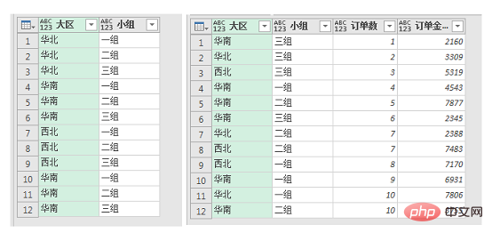
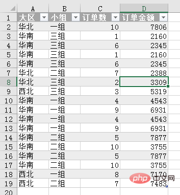
The case is as shown in the figure. There are two worksheets in the workbook, namely sales group and sales. Now we need to divide the "sales" table according to the region and group. The order number and order amount in are matched to the "Sales Group" table.

is a typical multi-condition query, which searches for data that meets multiple conditions and returns multiple columns of data.
Since the regions and groups in the two tables cannot be used as unique values for the search, it is necessary to search and match based on the two items, and the order number and order amount columns must be matched. It would be too brain-consuming to implement this using a function. How to do it? The steps are as follows:
1. Click on the Data tab, New Query - From File - From Workbook.

2. Find the workbook in the "Import Data" window and click Import.

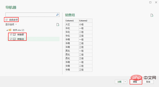
3. Click "Multiple Select" in the "Navigator" window, then select two worksheets and click "Edit".
After entering the Power Query editor, you can see the two imported worksheet queries in the query window on the left.
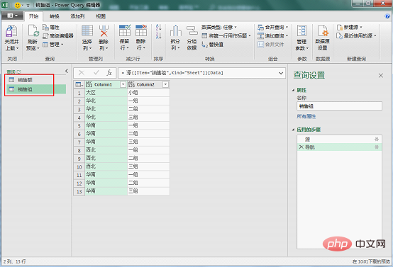
#4. Since the imported table uses column as the new title, in order to facilitate future operations, we first use the first row of the two queries as the title. Click on both queries and click "Use first row as title" under the Home tab.

Complete as follows:
5. Next, perform a merge query of the two tables. Select the table "Sales Group" where you want to fill in the content, and click "Merge Query into New Query" in the "Merge Query" drop-down menu under the Home tab.

6. In the "Merge Window", the first table is the table "Sales Group" to be filled in with matching content, and the second table containing matching information is selected in the drop-down window. Table "Sales". First, select the "large area" column of the two tables, and the two columns will turn green. This means that the two tables match data through the "region" column.
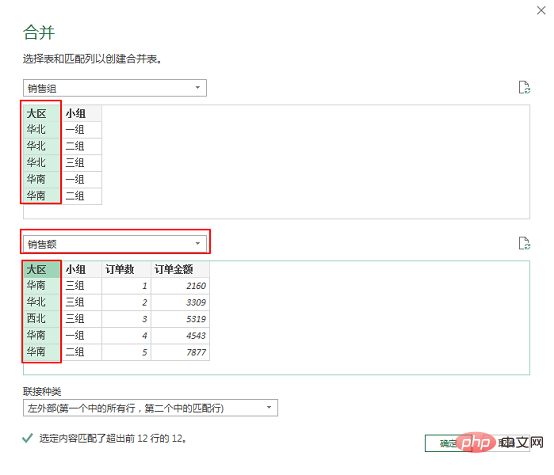
Then hold down the Ctrl key and select the "Group" column of the two tables again. At this time, the two table column labels "1" and "2" appear. Where 1 column matches 1 column and 2 columns matches 2 columns. Click OK.
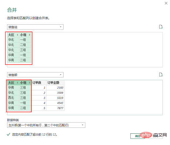
Note: There are six types of connection types below. We choose the first "left outer", that is, the values in the first table are unique values. According to the selected columns to join all rows in the first table to matching rows in the second table. That is the function of our commonly used VLOOKUP. The merged query here selects the first type by default. If you are interested, we can introduce the other five connection types later.

7. The query window will generate a new query "Merge1", and the information in the "Sales" table will be matched in the new query table. Click the table in the sales column to preview. In the preview pane below, you can see all the contents of the sales table matched based on the same region and group.
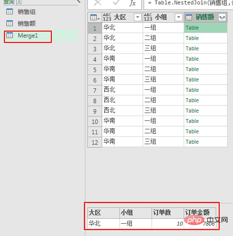
Using this method, we can freely select the number of matching columns in the merge window, 2 columns, 3 columns or even more columns can be satisfied. This solves the problem of multi-condition search; and all contents of the matching table can be found according to the matching columns.
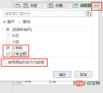
8. Now expand the content that needs to be imported into the table. Click the expand button to the right of the "Sales" column. In the expansion pane below, select the columns "Number of Orders" and "Order Amount" to be expanded. Do not check "Use original column name as prefix".
Complete as follows:
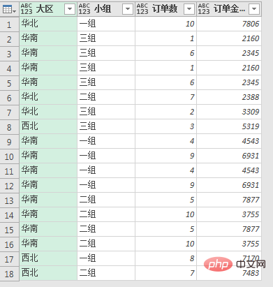
9.Finally upload this query to the form. Select the new query table and click "Close and Upload" under the Home tab.

This will upload all three query tables to the workbook and generate three new worksheets. The "Workbook Query" window will appear on the right. Click on the new query and the workbook will automatically jump to the corresponding query worksheet.

Complete as follows:
Okay, this is the end of the introduction to the merge query of Power Query. This query method connects two tables based on multiple matching columns and matches the tables. It is very helpful for complex multi-table queries in daily work. If you are interested, please leave me a message!
Related learning recommendations: excel tutorial
The above is the detailed content of Practical Excel skills sharing: merge query to achieve multi-table search and matching for various requirements at one time. For more information, please follow other related articles on the PHP Chinese website!

Hot AI Tools

Undresser.AI Undress
AI-powered app for creating realistic nude photos

AI Clothes Remover
Online AI tool for removing clothes from photos.

Undress AI Tool
Undress images for free

Clothoff.io
AI clothes remover

AI Hentai Generator
Generate AI Hentai for free.

Hot Article
Hot Tools

Notepad++7.3.1
Easy-to-use and free code editor

SublimeText3 Chinese version
Chinese version, very easy to use

Zend Studio 13.0.1
Powerful PHP integrated development environment

Dreamweaver CS6
Visual web development tools

SublimeText3 Mac version
God-level code editing software (SublimeText3)
Hot Topics
 1386
1386
 52
52

 What should I do if the frame line disappears when printing in Excel?
Mar 21, 2024 am 09:50 AM
What should I do if the frame line disappears when printing in Excel?
Mar 21, 2024 am 09:50 AM
If when opening a file that needs to be printed, we will find that the table frame line has disappeared for some reason in the print preview. When encountering such a situation, we must deal with it in time. If this also appears in your print file If you have questions like this, then join the editor to learn the following course: What should I do if the frame line disappears when printing a table in Excel? 1. Open a file that needs to be printed, as shown in the figure below. 2. Select all required content areas, as shown in the figure below. 3. Right-click the mouse and select the "Format Cells" option, as shown in the figure below. 4. Click the “Border” option at the top of the window, as shown in the figure below. 5. Select the thin solid line pattern in the line style on the left, as shown in the figure below. 6. Select "Outer Border"
 How to filter more than 3 keywords at the same time in excel
Mar 21, 2024 pm 03:16 PM
How to filter more than 3 keywords at the same time in excel
Mar 21, 2024 pm 03:16 PM
Excel is often used to process data in daily office work, and it is often necessary to use the "filter" function. When we choose to perform "filtering" in Excel, we can only filter up to two conditions for the same column. So, do you know how to filter more than 3 keywords at the same time in Excel? Next, let me demonstrate it to you. The first method is to gradually add the conditions to the filter. If you want to filter out three qualifying details at the same time, you first need to filter out one of them step by step. At the beginning, you can first filter out employees with the surname "Wang" based on the conditions. Then click [OK], and then check [Add current selection to filter] in the filter results. The steps are as follows. Similarly, perform filtering separately again
 How to change excel table compatibility mode to normal mode
Mar 20, 2024 pm 08:01 PM
How to change excel table compatibility mode to normal mode
Mar 20, 2024 pm 08:01 PM
In our daily work and study, we copy Excel files from others, open them to add content or re-edit them, and then save them. Sometimes a compatibility check dialog box will appear, which is very troublesome. I don’t know Excel software. , can it be changed to normal mode? So below, the editor will bring you detailed steps to solve this problem, let us learn together. Finally, be sure to remember to save it. 1. Open a worksheet and display an additional compatibility mode in the name of the worksheet, as shown in the figure. 2. In this worksheet, after modifying the content and saving it, the dialog box of the compatibility checker always pops up. It is very troublesome to see this page, as shown in the figure. 3. Click the Office button, click Save As, and then
 How to type subscript in excel
Mar 20, 2024 am 11:31 AM
How to type subscript in excel
Mar 20, 2024 am 11:31 AM
eWe often use Excel to make some data tables and the like. Sometimes when entering parameter values, we need to superscript or subscript a certain number. For example, mathematical formulas are often used. So how do you type the subscript in Excel? ?Let’s take a look at the detailed steps: 1. Superscript method: 1. First, enter a3 (3 is superscript) in Excel. 2. Select the number "3", right-click and select "Format Cells". 3. Click "Superscript" and then "OK". 4. Look, the effect is like this. 2. Subscript method: 1. Similar to the superscript setting method, enter "ln310" (3 is the subscript) in the cell, select the number "3", right-click and select "Format Cells". 2. Check "Subscript" and click "OK"
 How to set superscript in excel
Mar 20, 2024 pm 04:30 PM
How to set superscript in excel
Mar 20, 2024 pm 04:30 PM
When processing data, sometimes we encounter data that contains various symbols such as multiples, temperatures, etc. Do you know how to set superscripts in Excel? When we use Excel to process data, if we do not set superscripts, it will make it more troublesome to enter a lot of our data. Today, the editor will bring you the specific setting method of excel superscript. 1. First, let us open the Microsoft Office Excel document on the desktop and select the text that needs to be modified into superscript, as shown in the figure. 2. Then, right-click and select the "Format Cells" option in the menu that appears after clicking, as shown in the figure. 3. Next, in the “Format Cells” dialog box that pops up automatically
 How to use the iif function in excel
Mar 20, 2024 pm 06:10 PM
How to use the iif function in excel
Mar 20, 2024 pm 06:10 PM
Most users use Excel to process table data. In fact, Excel also has a VBA program. Apart from experts, not many users have used this function. The iif function is often used when writing in VBA. It is actually the same as if The functions of the functions are similar. Let me introduce to you the usage of the iif function. There are iif functions in SQL statements and VBA code in Excel. The iif function is similar to the IF function in the excel worksheet. It performs true and false value judgment and returns different results based on the logically calculated true and false values. IF function usage is (condition, yes, no). IF statement and IIF function in VBA. The former IF statement is a control statement that can execute different statements according to conditions. The latter
 Where to set excel reading mode
Mar 21, 2024 am 08:40 AM
Where to set excel reading mode
Mar 21, 2024 am 08:40 AM
In the study of software, we are accustomed to using excel, not only because it is convenient, but also because it can meet a variety of formats needed in actual work, and excel is very flexible to use, and there is a mode that is convenient for reading. Today I brought For everyone: where to set the excel reading mode. 1. Turn on the computer, then open the Excel application and find the target data. 2. There are two ways to set the reading mode in Excel. The first one: In Excel, there are a large number of convenient processing methods distributed in the Excel layout. In the lower right corner of Excel, there is a shortcut to set the reading mode. Find the pattern of the cross mark and click it to enter the reading mode. There is a small three-dimensional mark on the right side of the cross mark.
 How to insert excel icons into PPT slides
Mar 26, 2024 pm 05:40 PM
How to insert excel icons into PPT slides
Mar 26, 2024 pm 05:40 PM
1. Open the PPT and turn the page to the page where you need to insert the excel icon. Click the Insert tab. 2. Click [Object]. 3. The following dialog box will pop up. 4. Click [Create from file] and click [Browse]. 5. Select the excel table to be inserted. 6. Click OK and the following page will pop up. 7. Check [Show as icon]. 8. Click OK.
