Excel function learning: CHOOSE function vs IF function

If there is a world in the Excel function circle, then the CHOOSE function can definitely be regarded as a sweeper. It is not as powerful as the IF function, but its capabilities are even better. Today Xiaohua will take you to have a good look at the CHOOSE function that has been ignored by most people!

1. Understand the basic statements of the CHOOSE function

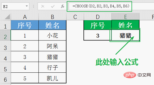
The CHOOSE function uses index_num Returns the numeric value in the numeric argument list. Use CHOOSE to select one of up to 254 values ​​based on an index number. Its basic statement is:

=CHOOSE(index_num,value1,value2,...)

index_num: parameter that specifies the index number, which is any integer between 1-254, CHOOSE selects the corresponding parameter from the parameter list value1 to value254 based on this value. index_num can be a number, formula, or cell reference. Please note the following two points when setting this parameter:

①If index_num is less than 1 or greater than the index number of the last value in the list, CHOOSE returns #VALUE! error value. For example, CHOOSE(3,1,2), since the index parameter is 3, but the parameter list has only two values, #VALUE! (Error type: The value cannot be found.)

②If index_num is decimal, it will be truncated before use. For example, CHOOSE(1.99,1,2), 1.99 is truncated and rounded to 1, then the first parameter value 1 is selected from the parameter list {1,2} as the formula return value.

Value1-value254: The parameter list contains at least one value parameter, that is, value1 is required, and the number of values ​​in the parameter list must be greater than or equal to the maximum possible value of index_num. value can be a number, cell reference, defined name, formula, function, or text.

2. Single logical judgment ability, CHOOSE must be inferior to IF.

After reading the statements and explanations of the above CHOOSE function, it is not difficult to find that the CHOOSE function It has the function of IF function.

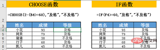
The basic statement of IF is IF (logical judgment, return value when the logic is correct, return value when the logic is wrong), plus TRUE corresponds to the value 1, FALSE corresponds to the value 0, so we can translate the IF function statement into CHOOSE Function statement, that is, CHOOSE (2-logical judgment value, return value when the logic is correct, return value when the logic is wrong).

When the logical judgment result is TRUE, 2-TRUE=2-1=1, the CHOOSE function selects value1 as the logical correct return value;

When the logical judgment result is FALSE, 2-FALSE= 2-0=2, the CHOOSE function selects value2 as the logical error return value.

Case:

Use the CHOOSE function and IF function to determine whether the score is qualified. The CHOOSE function needs to use 2-logical values ​​to convert the logical values ​​into index numbers, which is a bit complicated!

3. Multiple condition judgment ability, CHOOSE is even better

For multiple condition judgment, loyal fans of the IF function will Use multiple nesting methods to handle this. But the result of this is that the function formula is long and cumbersome, making it difficult to interpret. During the nesting process, we need to use the IF function multiple times. It is simpler to use the CHOOSE function to complete multiple conditional judgments, but you need to understand and master the setting principle of the index parameter index_num. Next, we will explain the principle of the multiple conditional judgment formula of the CHOOSE function with examples.

Case:

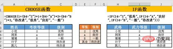
Convert the assessment level in the picture below into the corresponding level. Each person has a unique assessment level.

If we use the IF function at this time, we need triple nesting. This is still a relatively simple situation in the front nest of the IF function. When the number of conditions increases, the complexity of the IF function nested formula will also increase. . The CHOOSE function formula does not need to be nested, just write index_num as 1, logical judgment 1*1, logical judgment 2*2... Logical judgment is in the form of n*n, and set value 1 to when all conditions are not met. "To be improved", other value values ​​​​and logical judgment conditions can be arranged in sequence.

The IF function formula is as follows:

=IF(I4="S","Excellent",IF(I4="A","Good",IF(I4="B", "General","To be improved")))

The CHOOSE function formula is as follows:

=CHOOSE(1 (B4="S")*1 (B4="A")*2 (B4="B")*3,"To be improved" , "Excellent", "Good", "General")

Formula description:

The first parameter index_num of the CHOOSE function represents the selected parameter The index number of the list. When all conditions are not met, all logical conditions return FALSE, 1 ∑ logical condition n*n=1 0=1, select value 1 as the final return value of the formula, so value 1 should be filled in all The target result when none of the conditions are met, in this case should be "to be improved";

When the first condition is met, the other conditions are not met, 1 ∑ Logical condition n*n=1 1* 1 0=2, select value 2, that is, "excellent" as the return value;

When the second condition is met, the other conditions are not met, 1 ∑ Logical condition n*n=1 0*1 1* 2 0=3, select value 3, which is "good", as the return value;

and so on.

Therefore, when the logical conditions do not include each other, the first parameter of the CHOOSE function should be expressed in the form of 1 ∑ logical condition n*n, and the order of the remaining parameters is value all false, value if logical 1 true ,value if logical 2 true......

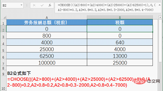
On the contrary, if the logical conditions are mutually inclusive, the first parameter index_num of the CHOOSE function should be written as 1 Logical judgment 1 Logical judgment 2... Logical judgment The form of n is 1 ∑ logical condition n. This is because when logic n is satisfied, logic n-1 must also be satisfied, so the number of satisfied conditions plus 1 is the index number of the selected parameter list, and there is no need to use the *n form for conversion. A typical problem is the tax calculation of labor remuneration income under the old personal income tax. For example, if the salary is 4,500 yuan, it is both greater than 4,000 and greater than 800. Add their logical values ​​and add 1 to get 3. The personal income tax is calculated using Value 3 in the formula, which is A2*0.8*0.2, as follows:

=CHOOSE(((A2>800) (A2>4000) (A2>25000) (A2>62500) 1),0,A2-800)*0.2,A2*0.8*0.2,A2*0.8*0.3-
2000,A2*0.8*0.4-7000)

4. Establish reverse search area capabilities, CHOOSE has an overall advantage

When using the VLOOKUP function for reverse lookup, we will use the IF{1,0} structure to complete the reconstruction of the table data columns, so that the target query value of VLOOKUP appears in the first column of the query range. For example, in the figure below, since the name column is on the right side of the grade column in the data source area, we cannot directly use VLOOKUP to query, so we use IF{1,0} to rearrange the data in columns A and C. When it is determined that True (1), output $C$10:$C$14 column data, judge as false (0) output $A$10:$A$14 column data, thus constructing a new column with $C$10:$C$14 as the first column, $A $10:$A$14 is the array in the second column as the search area, so that the VLOOKUP function can successfully query the target result.

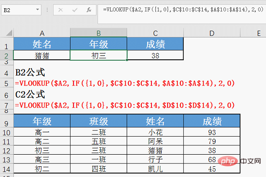
So, here comes the problem. The IF{1,0} structure can only specify the order of two columns of data, and cannot specify the order of multiple columns of data to combine into a new query area. This makes us often need to separate multiple cells of different query columns for the same query logic. Set the formula and cannot drag the fill formula to match the column lookup. For example, it is currently not possible to drag and fill the B2 formula into C2. This flaw in the IF{1,0} structure caused it to completely fail in comparison with CHOOSE!

The following is CHOOSE's approach, which directly reorders the three columns of data at once to build a unified query area. The formula can be directly dragged and filled from B2 to C2:

=VLOOKUP($A2 ,CHOOSE({1,2,3},$C$10:$C$14,$A$10:$A$14,$D$10:$D$14),COLUMN(),0)

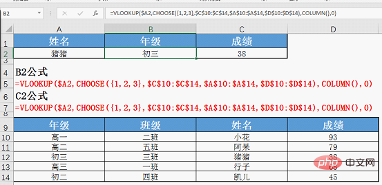
Formula description:

The key point of this formula is that we use the CHOOSE{1,2,3} structure to rearrange the three columns of data A10:A14, C10:C14, D10:$D14 in the table into column 1 and A10:A14 according to C10:C14 The order of column 2, D10:$D14 and column 3 forms a new data area used as the Vlookup search area. Then use COLUMN() to return the number of columns in the cell where the formula is located to determine the number of columns returned by the VLOOKUP query. This usage of the CHOOSE function greatly breaks through the limitation that the IF{1,0} structure can only exchange the positions of two columns of data for reconstruction. It can be said to be an enhanced version of the latter!

In this article, Xiaohua explains several practical usages of CHOOSE through a horizontal comparison of the CHOOSE function and the IF function. Have you learned these usages? What other skills do you know related to the CHOOSE function? Don’t forget to leave a message to communicate and share with Xiaohua!

Related learning recommendations: excel tutorial

The above is the detailed content of Excel function learning: CHOOSE function vs IF function. For more information, please follow other related articles on the PHP Chinese website!