Practical Excel skills sharing: 7 practical positioning skills to help you improve work efficiency

The positioning function in Excel is very powerful, but many newcomers in the workplace can only locate blank spaces. In fact, it also has many very useful functions. Today I will share with you 7 Excel positioning skills.

Tip 1: Quickly fill across rows

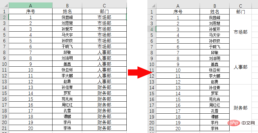
The following table is a table of department information for employees of a company. Now you need to fill in the blank cells in the department column Fill based on the top cell.

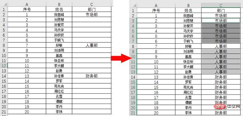
#In the above situation, if there is not much content, just drag the mouse to fill it in quickly. If there is a lot of content, our first priority would be to use Ctrl+G to locate the space and then quickly fill it in.

Operation steps:

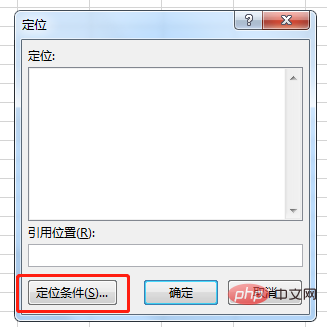
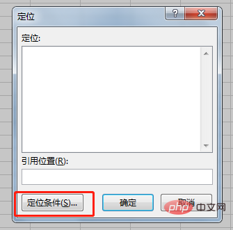
(1) Select the C1:C21 data area and press the Ctrl G shortcut key, click [Positioning Conditions], and single-select the [Null Value] option.

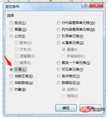
(2) Click [OK] and the blank cells in the C1:C21 area have been selected.

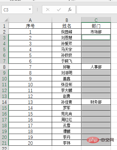
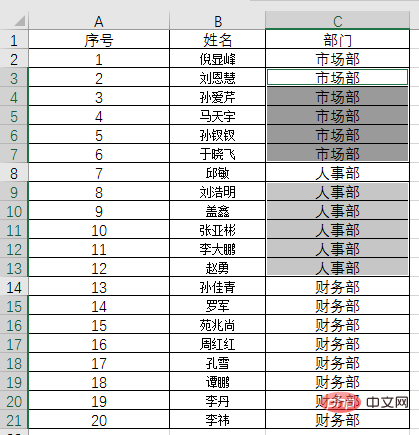
(3) Enter =C2 in the edit bar and press the shortcut key Ctrl Enter to fill all the blank cells.

Tip 2: Quickly merge the same cells

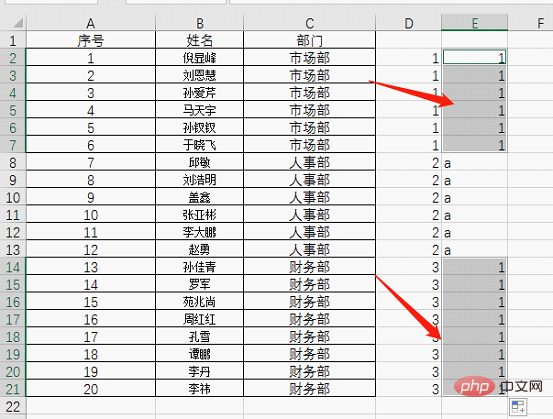
This technique is suitable for situations where there is a lot of data, such as hundreds or thousands of rows of data. Merge identical cells in the same column.

Operation steps:

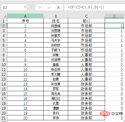
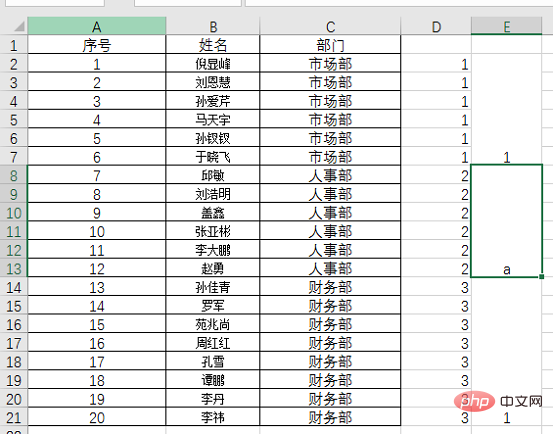
(1) Use D as the auxiliary column, and enter the function =IF(C2=C1,D1,D1 in unit D2 1), the purpose is to label the same departments.

(2) With column E as the auxiliary column, enter the function formula =IF(-1^D2>0,"a",1) in cell E2. The meaning of the formula is that by calculating -1 raised to the 1st power is -1 and -1 raised to the 2nd power is 1, the results obtained are -1 and 1. Then use the IF function to distinguish it into numbers and text forms such as 1 and a.

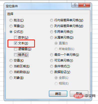
# (3) Use the CTRL G shortcut key to open the [Location Conditions] dialog box.

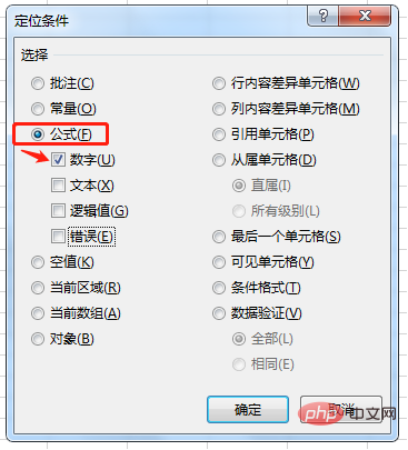
(4) In the [Positioning Conditions] dialog box, select [Number] in [Formula] and click OK.

(5) Select the number in column E, and then click the [Merge and Center] function.

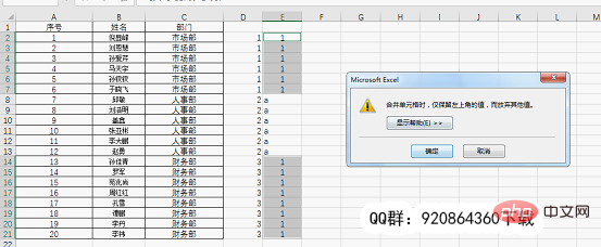
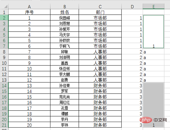
(6) Locate the text content in column E again, and do the same after selecting the cell Click the [Merge and Center] function.

(7) After completing the merger of column E, select column E, click the format painter, and format the target cell in column C. Refresh.

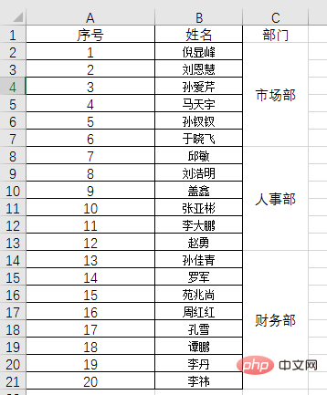
In this way, we have completed the merging of the same cells. You can try to demonstrate the operation yourself.

Technique 3: Number Batch Color Marking

The following table is the employee assessment score information table. Now we need to mark all scores in red.

Operation steps:

(1) After selecting the entire table, use the CTRL G shortcut key to open the positioning dialog box, and click [Positioning Conditions].

(3) Open the [Positioning Conditions] dialog box, click [Constant], we see that the check box below becomes selectable, check the number Selected.

Click [OK], and all the numbers in the table will be selected.

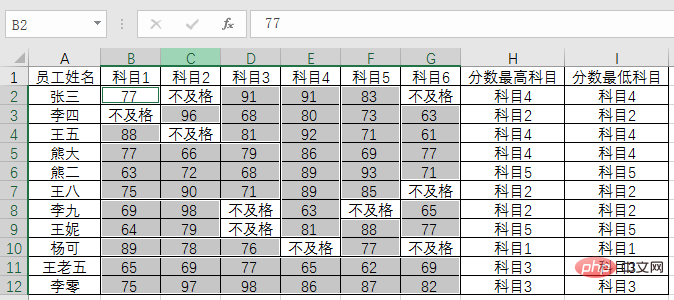
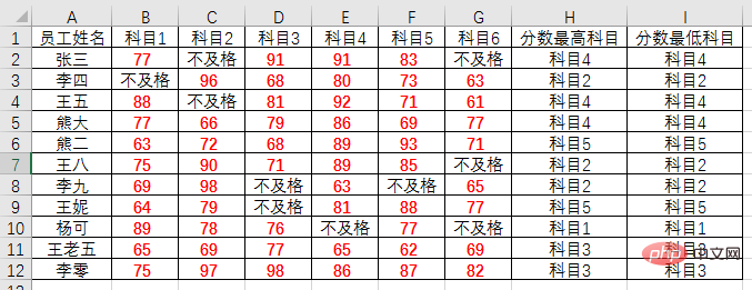
(4) Set the text color and complete the digital color marking.

Tip 4: Delete comments in batches

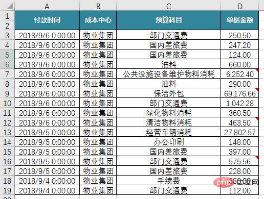
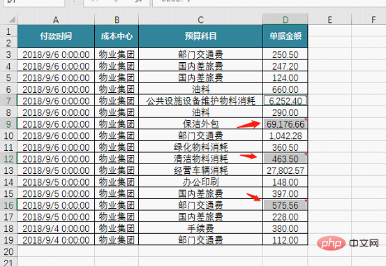
The following table is a detailed list of expenses for a certain property formula. There are comments in part of the data in the document amount, which are now needed Delete all comments.

Operation steps:

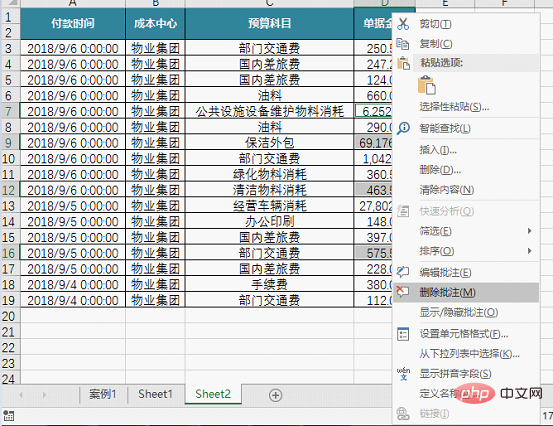
(1) After selecting the entire table, use the CTRL G shortcut key to open the [Location Conditions] dialog box and select annotation.

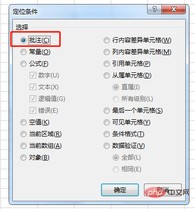
Click "OK" and we see three cells with comments selected.

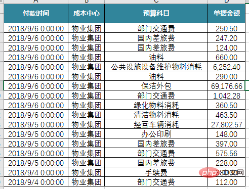
# (2) Right-click the mouse and select "Delete Comment" to complete.

Tip 5: Quickly find the difference in row/column content

The positioning function can also quickly compare two rows ( The difference between the contents of multiple rows) or two columns (multiple columns). The teacher's answers and accounting reconciliations are very useful.

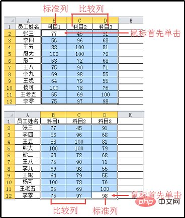
How to compare? One row (column) serves as the standard and the others serve as comparison rows (columns). The standard row (column) is the row (column) of the cell where the mouse first clicks when selecting data.

Standard rows                                                                                                                                                                                                                                                  .

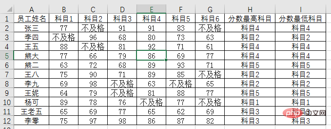
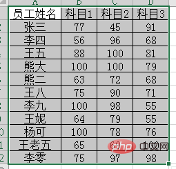
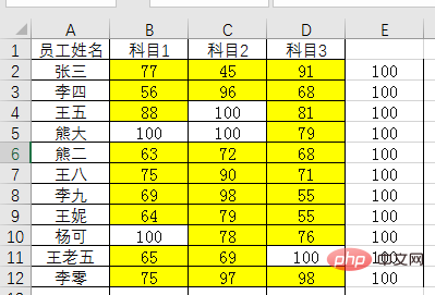
The following table is the employee test score information table for three subjects. We need to quickly mark the cells that are not 100 in each subject in yellow.

1) Quick row difference comparison ctrl shift

(1) Enter 100 in cell B13:D13 as an auxiliary cell , select the table data area from the bottom right to the top.

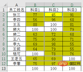
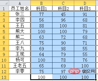(2) Press the shortcut key ctrl shift

to select cells other than 100 and then color them.

2) Quick column difference comparison ctrl

(1) Add auxiliary data 100 in column E on the right side of the data area, from Select the data area from right to left.

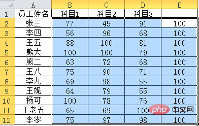(2) Press the shortcut key ctrl

to select cells other than 100 and then color them.

Tip 6: Quickly sort out wrong row data

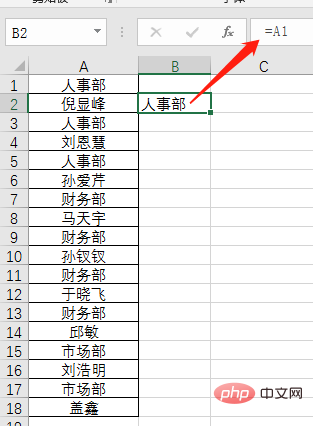
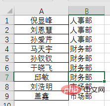
The data in column A in the table below shows department information and name information in alternate rows. Now we need to sort it out. Have a separate column for names and a separate column for department information.

Operation steps:

(1) First enter =A1 cell in cell B2, then select cells B1:B2 and copy and fill downwards .

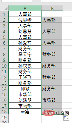(2) Press CTRL G to open the positioning conditions and select the null value in the positioning conditions.

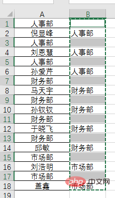
(3) Right-click the mouse and select "Delete" to delete the entire line.

Tip 7: Batch delete objects (including charts, pictures, shapes, smartart)

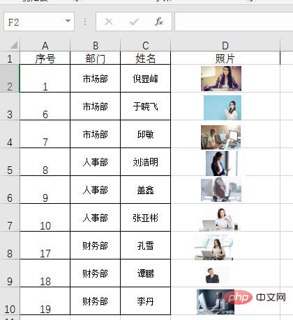
We often encounter objects when using excel worksheets daily, such as Shapes, pictures, charts, smartart, etc. If you need to delete these objects at once, you can use Ctrl G. The following table is the basic information of employees, in which photos are inserted into the table as objects. We can complete the photo deletion operation through positioning.

Operation steps:

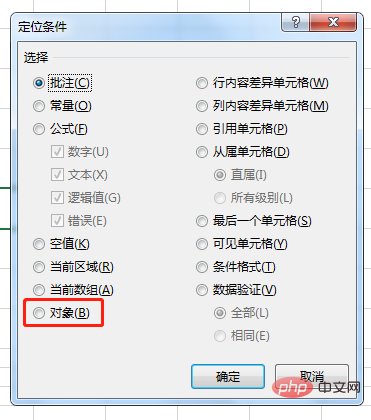
(1) Use the Ctrl G shortcut key to open the [Positioning] dialog box, click [Positioning Conditions] to open the Positioning Conditions dialog box , select [Object].

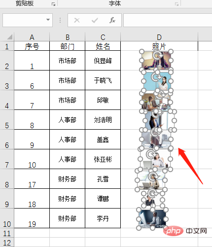
(2) After clicking [OK], we see that all the photos are selected. At this time, we only need to press delete to complete the deletion of the object photos.

Summary

In this tutorial, we have shared 7 practical positioning skills with you. We hope that these 7 skills can help you quickly improve your work efficiency.

Related learning recommendations: excel tutorial

The above is the detailed content of Practical Excel skills sharing: 7 practical positioning skills to help you improve work efficiency. For more information, please follow other related articles on the PHP Chinese website!