

Practical Excel skills sharing: 3 ways to quickly extract cell data

How to quickly extract cell data in Excel? The following article summarizes 3 extraction methods for you, ranging from the simplest shortcut key operations to the imaginative space replacement method. Extracting cell data can only use 99 spaces! I really want to pry open the heads of some great gods to see how they get along with each other in such incredible ways.

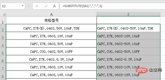
It is necessary to extract three sets of data of capacitance, packaging and voltage resistance from the specifications and models, as follows:
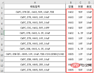
The data source is in column A. The amount of data is very large. The byte positions of the three data that need to be extracted, namely capacitance, packaging and voltage resistance, are not fixed in the cell. The rule that can be found is that the extracted data is located after the second, third, and fourth commas of the data source.
When we encounter a problem, finding the pattern is the key to solving the problem. Now that the pattern is found, so is the solution. There are three methods here, ranging from the simplest shortcut key operation to the imaginative space replacement method. They are introduced below.
1. Quick filling method Ctrl E
Operation points:
(1) Enter in cell B2 At 0402, enter a single quote first, or change the cell to text format before entering;
(2) Entering only one data may not get the correct result through Ctrl E. At this time, enter two data continuously. That's it.
Tip: The key combination Ctrl E can only be used in Excel 2013 and above.
As far as this example is concerned, Ctrl E is a little troublesome, so I will introduce another method of using columns.
2. Column separation method
Operation points:
(1) Use commas in the column separation process Separate;
(2) You need to skip the columns that are not imported;
(3) Set the data in the value column to text format;
(4) Manually Specify the target area for data storage.
Compared with the first method, using sorting is much simpler. At the same time, through this example, everyone can also have an in-depth understanding of the powerful function of sorting.
Although it is more convenient to use columns, if you often need to process this kind of data, the amount of operations is quite large. Finally, we will share a formula method.
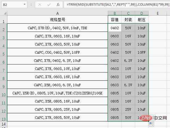
3. Brainstorm: TRIM-MID-SUBSTITUTE-REPT combination formula
Use the formula: =TRIM(MID(SUBSTITUTE($A2 ,",",REPT("
",99)),COLUMN(B1)*99,99))
Pull down to the right to get the desired result.
Formula analysis:
Five functions are used in this formula, including the MID and COLUMN that we are more familiar with, and the TRIM, SUBSTITUTE and REPT functions that we are less commonly used. Let’s briefly explain this formula Idea.
The core part of the formula is SUBSTITUTE($A2,",",REPT(" ",99)). The function of this part is to replace.
The format of the SUBSTITUTE function is:
SUBSTITUTE(在哪里替换,替换什么,换成什么,换第几个)
For example:
Formula=SUBSTITUTE($A2,",","-",3)The effect is to replace the third comma in cell A2 Replace with - sign.
When the fourth parameter is omitted, it means that all commas are replaced, as shown in the figure:
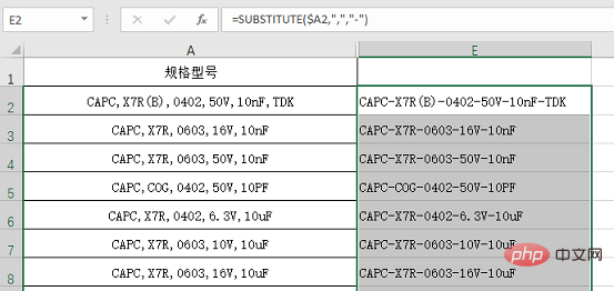
In this example, the commas in A2 are replaced by REPT(" ",99), which is 99 spaces.
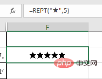
The format of the REPT function is:
REPT(要重复的字符,重复次数)
For example:
REPT(“★”,5) means repeating ★ five times.
As for why 99 spaces are used in the formula , is completely a routine. You may understand it if you continue to read the other parts of the formula.
The data obtained using SUBSTITUTE also needs to be extracted using the MID function. Everyone should be familiar with the MID function. The basic format is : MID (data source, where to start taking, how many words to take). In this example, the data source to be extracted is SUBSTITUTE(), and the location of the value to be extracted is originally after the second comma, because We replaced the comma with 99 spaces. There are at least two sets of spaces in front of the position to be extracted, which is 2*99 characters; the extracted position of the corresponding package is 3*99, and the pressure-resistant one is 4*99. Use the formula right Pull, so COLUMN(B1)*99 is used as the extraction position here. The last parameter of MID is to extract several characters. For the sake of safety, 99 characters are extracted uniformly.
In other words, after the calculation of the MID (SUBSTITUTE (), COLUMN (B1) * 99, 99) part of the formula, the result is that the capacity data we actually need is included in the preceding and following spaces. In order to facilitate everyone's understanding, temporarily replace the spaces with -, and you can intuitively see the effect:
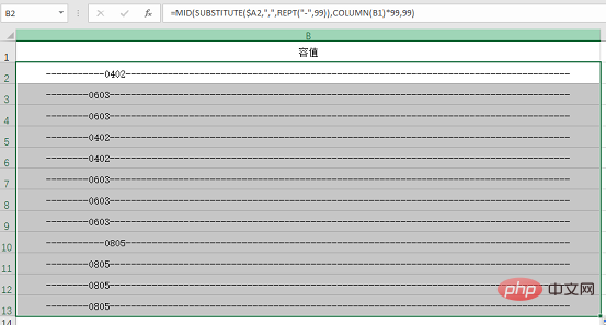
We definitely don't want the results to contain a large number of useless spaces, so Set a TRIM function in the outermost layer to remove these spaces. The TRIM function has only one parameter, and its function is to remove extra spaces in the string.
Related learning recommendations: excel tutorial
The above is the detailed content of Practical Excel skills sharing: 3 ways to quickly extract cell data. For more information, please follow other related articles on the PHP Chinese website!

Hot AI Tools

Undresser.AI Undress
AI-powered app for creating realistic nude photos

AI Clothes Remover
Online AI tool for removing clothes from photos.

Undress AI Tool
Undress images for free

Clothoff.io
AI clothes remover

AI Hentai Generator
Generate AI Hentai for free.

Hot Article
Hot Tools

Notepad++7.3.1
Easy-to-use and free code editor

SublimeText3 Chinese version
Chinese version, very easy to use

Zend Studio 13.0.1
Powerful PHP integrated development environment

Dreamweaver CS6
Visual web development tools

SublimeText3 Mac version
God-level code editing software (SublimeText3)
Hot Topics
 1378
1378
 52
52

 What should I do if the frame line disappears when printing in Excel?
Mar 21, 2024 am 09:50 AM
What should I do if the frame line disappears when printing in Excel?
Mar 21, 2024 am 09:50 AM
If when opening a file that needs to be printed, we will find that the table frame line has disappeared for some reason in the print preview. When encountering such a situation, we must deal with it in time. If this also appears in your print file If you have questions like this, then join the editor to learn the following course: What should I do if the frame line disappears when printing a table in Excel? 1. Open a file that needs to be printed, as shown in the figure below. 2. Select all required content areas, as shown in the figure below. 3. Right-click the mouse and select the "Format Cells" option, as shown in the figure below. 4. Click the “Border” option at the top of the window, as shown in the figure below. 5. Select the thin solid line pattern in the line style on the left, as shown in the figure below. 6. Select "Outer Border"
 How to filter more than 3 keywords at the same time in excel
Mar 21, 2024 pm 03:16 PM
How to filter more than 3 keywords at the same time in excel
Mar 21, 2024 pm 03:16 PM
Excel is often used to process data in daily office work, and it is often necessary to use the "filter" function. When we choose to perform "filtering" in Excel, we can only filter up to two conditions for the same column. So, do you know how to filter more than 3 keywords at the same time in Excel? Next, let me demonstrate it to you. The first method is to gradually add the conditions to the filter. If you want to filter out three qualifying details at the same time, you first need to filter out one of them step by step. At the beginning, you can first filter out employees with the surname "Wang" based on the conditions. Then click [OK], and then check [Add current selection to filter] in the filter results. The steps are as follows. Similarly, perform filtering separately again
 How to change excel table compatibility mode to normal mode
Mar 20, 2024 pm 08:01 PM
How to change excel table compatibility mode to normal mode
Mar 20, 2024 pm 08:01 PM
In our daily work and study, we copy Excel files from others, open them to add content or re-edit them, and then save them. Sometimes a compatibility check dialog box will appear, which is very troublesome. I don’t know Excel software. , can it be changed to normal mode? So below, the editor will bring you detailed steps to solve this problem, let us learn together. Finally, be sure to remember to save it. 1. Open a worksheet and display an additional compatibility mode in the name of the worksheet, as shown in the figure. 2. In this worksheet, after modifying the content and saving it, the dialog box of the compatibility checker always pops up. It is very troublesome to see this page, as shown in the figure. 3. Click the Office button, click Save As, and then
 How to type subscript in excel
Mar 20, 2024 am 11:31 AM
How to type subscript in excel
Mar 20, 2024 am 11:31 AM
eWe often use Excel to make some data tables and the like. Sometimes when entering parameter values, we need to superscript or subscript a certain number. For example, mathematical formulas are often used. So how do you type the subscript in Excel? ?Let’s take a look at the detailed steps: 1. Superscript method: 1. First, enter a3 (3 is superscript) in Excel. 2. Select the number "3", right-click and select "Format Cells". 3. Click "Superscript" and then "OK". 4. Look, the effect is like this. 2. Subscript method: 1. Similar to the superscript setting method, enter "ln310" (3 is the subscript) in the cell, select the number "3", right-click and select "Format Cells". 2. Check "Subscript" and click "OK"
 How to set superscript in excel
Mar 20, 2024 pm 04:30 PM
How to set superscript in excel
Mar 20, 2024 pm 04:30 PM
When processing data, sometimes we encounter data that contains various symbols such as multiples, temperatures, etc. Do you know how to set superscripts in Excel? When we use Excel to process data, if we do not set superscripts, it will make it more troublesome to enter a lot of our data. Today, the editor will bring you the specific setting method of excel superscript. 1. First, let us open the Microsoft Office Excel document on the desktop and select the text that needs to be modified into superscript, as shown in the figure. 2. Then, right-click and select the "Format Cells" option in the menu that appears after clicking, as shown in the figure. 3. Next, in the “Format Cells” dialog box that pops up automatically
 How to use the iif function in excel
Mar 20, 2024 pm 06:10 PM
How to use the iif function in excel
Mar 20, 2024 pm 06:10 PM
Most users use Excel to process table data. In fact, Excel also has a VBA program. Apart from experts, not many users have used this function. The iif function is often used when writing in VBA. It is actually the same as if The functions of the functions are similar. Let me introduce to you the usage of the iif function. There are iif functions in SQL statements and VBA code in Excel. The iif function is similar to the IF function in the excel worksheet. It performs true and false value judgment and returns different results based on the logically calculated true and false values. IF function usage is (condition, yes, no). IF statement and IIF function in VBA. The former IF statement is a control statement that can execute different statements according to conditions. The latter
 Where to set excel reading mode
Mar 21, 2024 am 08:40 AM
Where to set excel reading mode
Mar 21, 2024 am 08:40 AM
In the study of software, we are accustomed to using excel, not only because it is convenient, but also because it can meet a variety of formats needed in actual work, and excel is very flexible to use, and there is a mode that is convenient for reading. Today I brought For everyone: where to set the excel reading mode. 1. Turn on the computer, then open the Excel application and find the target data. 2. There are two ways to set the reading mode in Excel. The first one: In Excel, there are a large number of convenient processing methods distributed in the Excel layout. In the lower right corner of Excel, there is a shortcut to set the reading mode. Find the pattern of the cross mark and click it to enter the reading mode. There is a small three-dimensional mark on the right side of the cross mark.
 How to insert excel icons into PPT slides
Mar 26, 2024 pm 05:40 PM
How to insert excel icons into PPT slides
Mar 26, 2024 pm 05:40 PM
1. Open the PPT and turn the page to the page where you need to insert the excel icon. Click the Insert tab. 2. Click [Object]. 3. The following dialog box will pop up. 4. Click [Create from file] and click [Browse]. 5. Select the excel table to be inserted. 6. Click OK and the following page will pop up. 7. Check [Show as icon]. 8. Click OK.
