Why does vlookup display formulas?
vlookup displays formulas because the cells that should display data are set to non-text format or because the formula option is checked to display formulas. The solution: 1. Find the cell that displays the formula, Then right-click and select "Format Cells"; 2. Change the non-conventional classification on the "Number" interface to "General" and click "OK" to save.

The operating environment of this tutorial: Windows 10 system, WPS Office 2019 version, Dell G3 computer.
Why does vlookup display formulas?
In fact, there are only two reasons why the vlookup function only displays formulas. The first point is that we set the cells that should display data to non-text format, and the second point is that we set the The formula option has Show formula checked. Below I will give you a solution to the problem from these two points.
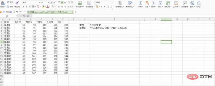
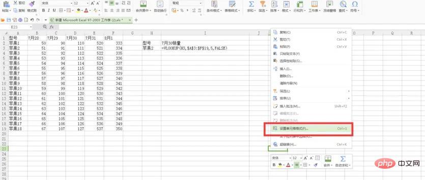
We find the cell that displays the formula, then right-click and select "Format Cells".
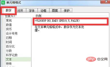
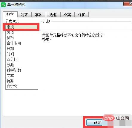
Then we change the non-conventional classification on the "Number" interface to "General" and click OK to save.
We switch to the form. At this time you will find that the data on the form has turned into numbers, so this means that we Already successful.
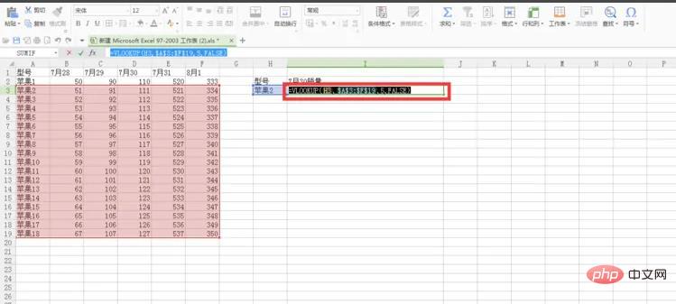
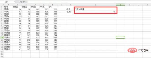
If it doesn’t work, you must be using an old version of the office software, but it’s not a big problem. Let’s choose the “ Formula" and then click "Show Formula" so that the vlookup function will not only display the formula. Isn't it very simple?
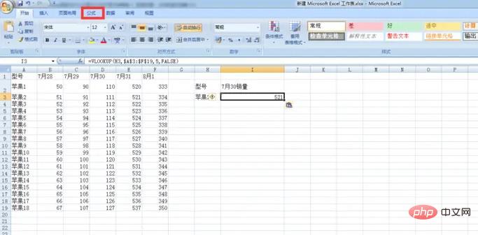
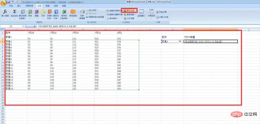
Excel Tutorial"
The above is the detailed content of Why does vlookup display formulas?. For more information, please follow other related articles on the PHP Chinese website!

Hot AI Tools

Undresser.AI Undress
AI-powered app for creating realistic nude photos

AI Clothes Remover
Online AI tool for removing clothes from photos.

Undress AI Tool
Undress images for free

Clothoff.io
AI clothes remover

AI Hentai Generator
Generate AI Hentai for free.

Hot Article

Hot Tools

Notepad++7.3.1
Easy-to-use and free code editor

SublimeText3 Chinese version
Chinese version, very easy to use

Zend Studio 13.0.1
Powerful PHP integrated development environment

Dreamweaver CS6
Visual web development tools

SublimeText3 Mac version
God-level code editing software (SublimeText3)

Hot Topics
 1378
1378
 52
52
 How to find data with the same name through vlookup function
Mar 03, 2023 am 10:33 AM
How to find data with the same name through the vlookup function: 1. Open an Excel worksheet with duplicate data; 2. Select cell "C2", then select insert function "fx", and then find "VLOOKUP" in the pop-up function parameters; 3. Find the same data through the formula "=VLOOKUP(A2,A3:A14,1,0)=A2".
 Why does vlookup display formulas?
Mar 02, 2023 pm 02:22 PM
Vlookup displays formulas because the cells that should display data are set to non-text format or because the formula option is checked to display formulas. The solution: 1. Find the cell that displays the formula, then right-click and select "Settings" Cell Format"; 2. Change the non-conventional classification on the "Number" interface to "General" and click "OK" to save.
 How does the vlookup function match two columns of data?
Aug 07, 2023 am 11:35 AM
The method for the vlookup function to match two columns of data: 1. Make sure that the two columns of data are located in two different areas, such as column A and column B; 2. In the cell where the result needs to be returned, enter the formula of the vlookup function, such as =VLOOKUP (A2, B:C, 2, FALSE), FALSE means an exact match, if you want an approximate match, you can change it to TRUE; 3. Press the Enter key to find and return the matching results.
 What should I do if the matching result of the vlookup function is N/A?
Aug 01, 2023 am 09:52 AM
The vlookup function matching result is N/A. Solution: 1. Check the data integrity and confirm whether the data range and value to be matched are complete; 2. Check whether the matching value exists, and carefully check the data type, format and format of the matching value and search range. Whether the upper and lower case are completely consistent; 3. Format the data type, you can try to convert the data type of the matching value to be consistent with the search range, or use other functions to convert; 4. Use the IFERROR function to handle errors and use the IFERROR function to replace the error value into other custom values or blank.
 What should I do if the vlookup function cannot match and only displays the formula?
Nov 14, 2022 am 10:49 AM
The solution to the problem that the vlookup function cannot match and only the formula is displayed: 1. Enter the Excel software interface; 2. Select the input vlookup function cell and double-click the cell; 3. Move the cursor to behind the single quotation mark at the front of the formula; 4. , click the delete key on the keyboard, delete the single quotes, and then click the enter key.
![[Organization and Sharing] 4 ways to use VLOOKUP and LOOKUP functions for fuzzy search](https://img.php.cn/upload/article/000/000/024/63fc89de9ab36136.jpg?x-oss-process=image/resize,m_fill,h_207,w_330) [Organization and Sharing] 4 ways to use VLOOKUP and LOOKUP functions for fuzzy search
Feb 27, 2023 pm 06:46 PM
[Organization and Sharing] 4 ways to use VLOOKUP and LOOKUP functions for fuzzy search
Feb 27, 2023 pm 06:46 PM
Most of the time we need to perform precise searches, but there are also times when fuzzy searches are needed. For example, searching for the full name based on the abbreviation, or classifying the name based on numerical values, etc. Fuzzy search is not the same as a blind man trying to find an elephant. Here are 4 ways to use VLOOKUP and LOOKUP functions to perform fuzzy search.
 How to use vlookup function
Jan 10, 2024 am 10:05 AM
Instructions for use: 1. Open the Excel table and select the cells where the function needs to be used; 2. Enter "=VLOOKUP(lookup_value, table_array, col_index_num, [range_lookup])"; 3. In the function, "lookup_value" is the value to be found , "table_array" is a table or area containing data...; 4. Press the Enter key to complete the calculation of the VLOOKUP function.
 How to use the vlookup function
Nov 17, 2023 am 10:17 AM
The VLOOKUP function is one of the most commonly used functions in Excel. It is used to find the position of a value in another table or range and return the value at that position. How to use it: 1. Open Excel and open the workbook where you want to use the VLOOKUP function; 2. In the cell where you want to enter the VLOOKUP function, enter "=VLOOKUP(lookup_value, table_array, col_index_num, [range_lookup])" and so on. .


