

How to use the MATCH() function in Excel function learning

Today we are going to talk about another family - Find the Family! Speaking of finding families, I believe the first thing that comes to mind is the VLOOKUP function. This eldest brother has been working hard in the battlefield for many years and has already become famous! I believe that friends who have been exposed to Excel have heard of it to some extent. However, what we are going to talk about today is its capable little brother - the MATCH function!

#This little brother, although his ability is not very good on his own, but when he forms a team with his big brother, the effect is quite impressive!

Let’s get to know him first
1. Who is MATCH?
MATCH is a search positioning function. What it returns is not the data itself, but the position of the data in a single column or row. It's similar to queuing up to report the number. Whichever number you stand on, MATCH the number you report! (Note: It only supports single column or single row data search~)
Function structure: MATCH (What to look for, where to find [single row or single column], search type)
Search type: 3 kind. They are represented by 0, 1, and -1 respectively. 0 indicates exact search, 1 indicates ascending search, and -1 indicates descending search.
2. Basic usage of MATCH
1. Search accurately
Give me a chestnut
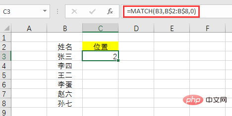
We want to know where "Zhang San" ranks in the "Name" column area.

Formula:
<strong>=MATCH(B3,B$2:B$8,0)</strong>
Formula analysis:
What to look for: Look for "Zhang San", so it is cell B3
Where to find it: Find it in the name column B2:B8. In order to prevent the name column area of the downward filling formula from changing, it needs to be fixed with $, that is, B$2:B$8.
Search type: 0 means precise search. Exact search does not require sorting.
2. Ascending search
Ascending search is to find the maximum value that is less than or equal to the search value and then return its location. The data must be sorted in ascending order.
Similarly give a chestnut
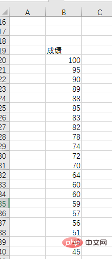
We want to know how many are no larger than 60.
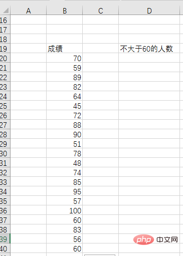
First sort the results in ascending order.
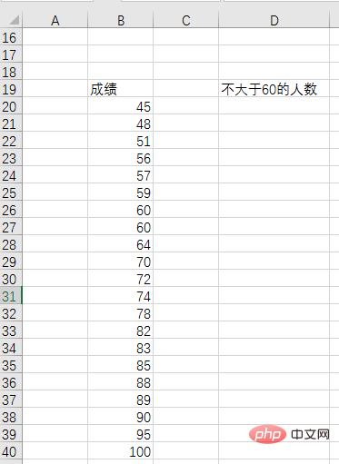
Then enter the formula in D3: =MATCH(60,B20:B40,1)
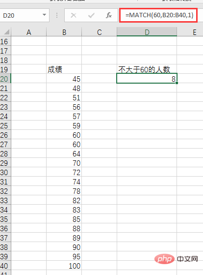
After confirmation, the number of people was 8. Obviously, after sorting in ascending order, what is returned is the position number of the last value less than or equal to 60; it can also be understood as counting the number of values not greater than 60, including all values equal to 60.
3. Descending search
Descending search is to find the minimum value that is greater than or equal to the search value and then return its location. Requirements must be sorted in descending order.
Similarly give a chestnut

We want to know how many are not less than 60. Following the above, first sort the data in descending order.
Then enter the formula in E3: =MATCH(60,B20:B40,-1)
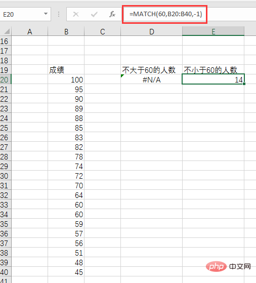
After confirmation, 14 people got no less than 60.
We got two obvious results:
(1) After descending order, an error occurs when searching in ascending order. Therefore, if you search in ascending order, you must sort in ascending order; conversely, if you search in descending order, you must sort in descending order.
(2) Descending search returns the smallest number greater than 60 or the number of positions of the first number equal to 60; it can also be understood as counting all numbers greater than 60 including the first number equal to 60 The number of values. This is different from filtering in ascending order: if there is a value that is the same as the search value, ascending order locates the last value equal to the search value, while descending order locates the first value equal to the search value.
After understanding who MATCH is and its basic usage, I guess everyone will think that MATCH is a bit useless: it is just used to return the position number, which is far from the specific value I want to find.
Because of this, the MATCH function rarely appears alone in daily work. MATCH is not discouraged. In order to win its place in the function world, it adopts an effective strategy-dancing with giants! Therefore, there are the famous VLOOKUP MATCH combination and INDEX MATCH combination.
3. Dancing with Giants
1. VLOOKUP MATCH combination
The following is a In a detailed list of scores, we need to find the total scores, average scores and grades of "Yuan Jingmi, Wang Hui, Lian Feng, and Yu Mai".
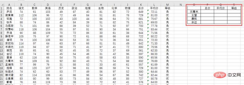
#If we use the VLOOKUP function alone, we need to frequently modify the third parameter. When checking the total score, enter the formula in cell P2:
=VLOOKUP(O2,A2:M142,11,0)
and you want to check the average score When , you need to modify the third parameter to 12, and the formula becomes:
=VLOOKUP(O2,A2:M142,12,0)
It is very convenient to use this way Trouble, how can we save trouble?
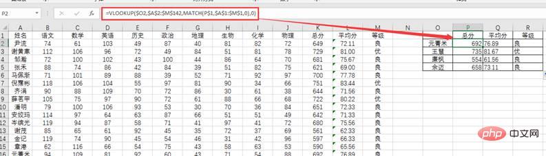
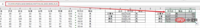
MACTH seized the opportunity to recommend itself to VLOOKUP, and replaced the third parameter with the position number of its own query "total score", "average score" and "level" in the A1:M1 row, so there is no need to modify it manually. At this time, the formula for finding the total score becomes:
=VLOOKUP($O2,$A$2:$M$142,MATCH(P$1,$A$1:$M$1,0), 0)
Then pull right to fill in and then pull down to fill in the formula to complete the query. As follows:
# Some friends may have seen our previous article "Can you use Column?" It makes the formula less dumb. ", saying that it is simpler to replace the third parameter with COLUMU:
=VLOOKUP($O2,$A$2:$M$142,COLUMN(K1),0)
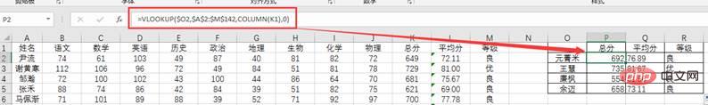
You are right. The current query values are arranged continuously, and the order is consistent with the order of the score details. It is easier to use COLUMN. What if the query is based on the following two tables?
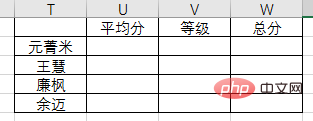
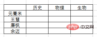
Obviously COLUMN is not suitable, but MATCH is fully qualified.
2. INDEX MATCH combination
Still check the results, as follows:
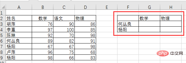
If we use INDEX alone to query scores, He Congliang’s math score query formula: =INDEX(A2:D9,5,2), physics score query formula: =INDEX(A2:D9,5,4).
INDEX query uses the specified query area as the coordinate system and queries the required values through row coordinates and column coordinates. The query area for He Congliang's grades is A2:D9, and the math score is located at the intersection of row 5 and column 2, so the formula is INDEX(A2:D9,5,2). The physics score is at the intersection of row 5 and column 4, so the formula is INDEX(A2:D9,5,4).
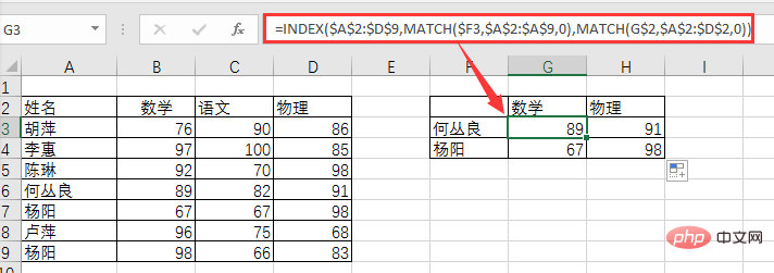
Querying by entering the number of rows and columns in this way is too clumsy and impractical. Therefore, MATCH took advantage of every opportunity to recommend itself to INDEX. MATCH can find the positioning value based on conditions, replacing the manual input of row and column numbers. The score query formula becomes:
=INDEX($A$2:$D$9,MATCH($F3,$A$2:$A$9,0),MATCH(G$2,$A$2 :$D$2,0))
Of course you can also use the VLOOKUP MATCH combination here, the formula:
=VLOOKUP($ F3,$A$2:$D$9,MATCH(G$2,$A$2:$D$2,0),0)
What is the difference between the VLOOKUP MATCH combination and the INDEX MATCH combination? We will discuss this issue in the subsequent function class. Interested partners can think about it themselves first.
How about it? Isn’t the combination of big brother and little brother great? Therefore, the MATCH function is worthy of being the philosopher among functions! That’s it for today’s function lesson, see you next time.
Related learning recommendations: excel tutorial
The above is the detailed content of How to use the MATCH() function in Excel function learning. For more information, please follow other related articles on the PHP Chinese website!

Hot AI Tools

Undresser.AI Undress
AI-powered app for creating realistic nude photos

AI Clothes Remover
Online AI tool for removing clothes from photos.

Undress AI Tool
Undress images for free

Clothoff.io
AI clothes remover

AI Hentai Generator
Generate AI Hentai for free.

Hot Article
Hot Tools

Notepad++7.3.1
Easy-to-use and free code editor

SublimeText3 Chinese version
Chinese version, very easy to use

Zend Studio 13.0.1
Powerful PHP integrated development environment

Dreamweaver CS6
Visual web development tools

SublimeText3 Mac version
God-level code editing software (SublimeText3)
Hot Topics
 1382
1382
 52
52

 What should I do if the frame line disappears when printing in Excel?
Mar 21, 2024 am 09:50 AM
What should I do if the frame line disappears when printing in Excel?
Mar 21, 2024 am 09:50 AM
If when opening a file that needs to be printed, we will find that the table frame line has disappeared for some reason in the print preview. When encountering such a situation, we must deal with it in time. If this also appears in your print file If you have questions like this, then join the editor to learn the following course: What should I do if the frame line disappears when printing a table in Excel? 1. Open a file that needs to be printed, as shown in the figure below. 2. Select all required content areas, as shown in the figure below. 3. Right-click the mouse and select the "Format Cells" option, as shown in the figure below. 4. Click the “Border” option at the top of the window, as shown in the figure below. 5. Select the thin solid line pattern in the line style on the left, as shown in the figure below. 6. Select "Outer Border"
 How to filter more than 3 keywords at the same time in excel
Mar 21, 2024 pm 03:16 PM
How to filter more than 3 keywords at the same time in excel
Mar 21, 2024 pm 03:16 PM
Excel is often used to process data in daily office work, and it is often necessary to use the "filter" function. When we choose to perform "filtering" in Excel, we can only filter up to two conditions for the same column. So, do you know how to filter more than 3 keywords at the same time in Excel? Next, let me demonstrate it to you. The first method is to gradually add the conditions to the filter. If you want to filter out three qualifying details at the same time, you first need to filter out one of them step by step. At the beginning, you can first filter out employees with the surname "Wang" based on the conditions. Then click [OK], and then check [Add current selection to filter] in the filter results. The steps are as follows. Similarly, perform filtering separately again
 How to change excel table compatibility mode to normal mode
Mar 20, 2024 pm 08:01 PM
How to change excel table compatibility mode to normal mode
Mar 20, 2024 pm 08:01 PM
In our daily work and study, we copy Excel files from others, open them to add content or re-edit them, and then save them. Sometimes a compatibility check dialog box will appear, which is very troublesome. I don’t know Excel software. , can it be changed to normal mode? So below, the editor will bring you detailed steps to solve this problem, let us learn together. Finally, be sure to remember to save it. 1. Open a worksheet and display an additional compatibility mode in the name of the worksheet, as shown in the figure. 2. In this worksheet, after modifying the content and saving it, the dialog box of the compatibility checker always pops up. It is very troublesome to see this page, as shown in the figure. 3. Click the Office button, click Save As, and then
 How to type subscript in excel
Mar 20, 2024 am 11:31 AM
How to type subscript in excel
Mar 20, 2024 am 11:31 AM
eWe often use Excel to make some data tables and the like. Sometimes when entering parameter values, we need to superscript or subscript a certain number. For example, mathematical formulas are often used. So how do you type the subscript in Excel? ?Let’s take a look at the detailed steps: 1. Superscript method: 1. First, enter a3 (3 is superscript) in Excel. 2. Select the number "3", right-click and select "Format Cells". 3. Click "Superscript" and then "OK". 4. Look, the effect is like this. 2. Subscript method: 1. Similar to the superscript setting method, enter "ln310" (3 is the subscript) in the cell, select the number "3", right-click and select "Format Cells". 2. Check "Subscript" and click "OK"
 How to set superscript in excel
Mar 20, 2024 pm 04:30 PM
How to set superscript in excel
Mar 20, 2024 pm 04:30 PM
When processing data, sometimes we encounter data that contains various symbols such as multiples, temperatures, etc. Do you know how to set superscripts in Excel? When we use Excel to process data, if we do not set superscripts, it will make it more troublesome to enter a lot of our data. Today, the editor will bring you the specific setting method of excel superscript. 1. First, let us open the Microsoft Office Excel document on the desktop and select the text that needs to be modified into superscript, as shown in the figure. 2. Then, right-click and select the "Format Cells" option in the menu that appears after clicking, as shown in the figure. 3. Next, in the “Format Cells” dialog box that pops up automatically
 How to use the iif function in excel
Mar 20, 2024 pm 06:10 PM
How to use the iif function in excel
Mar 20, 2024 pm 06:10 PM
Most users use Excel to process table data. In fact, Excel also has a VBA program. Apart from experts, not many users have used this function. The iif function is often used when writing in VBA. It is actually the same as if The functions of the functions are similar. Let me introduce to you the usage of the iif function. There are iif functions in SQL statements and VBA code in Excel. The iif function is similar to the IF function in the excel worksheet. It performs true and false value judgment and returns different results based on the logically calculated true and false values. IF function usage is (condition, yes, no). IF statement and IIF function in VBA. The former IF statement is a control statement that can execute different statements according to conditions. The latter
 Where to set excel reading mode
Mar 21, 2024 am 08:40 AM
Where to set excel reading mode
Mar 21, 2024 am 08:40 AM
In the study of software, we are accustomed to using excel, not only because it is convenient, but also because it can meet a variety of formats needed in actual work, and excel is very flexible to use, and there is a mode that is convenient for reading. Today I brought For everyone: where to set the excel reading mode. 1. Turn on the computer, then open the Excel application and find the target data. 2. There are two ways to set the reading mode in Excel. The first one: In Excel, there are a large number of convenient processing methods distributed in the Excel layout. In the lower right corner of Excel, there is a shortcut to set the reading mode. Find the pattern of the cross mark and click it to enter the reading mode. There is a small three-dimensional mark on the right side of the cross mark.
 How to insert excel icons into PPT slides
Mar 26, 2024 pm 05:40 PM
How to insert excel icons into PPT slides
Mar 26, 2024 pm 05:40 PM
1. Open the PPT and turn the page to the page where you need to insert the excel icon. Click the Insert tab. 2. Click [Object]. 3. The following dialog box will pop up. 4. Click [Create from file] and click [Browse]. 5. Select the excel table to be inserted. 6. Click OK and the following page will pop up. 7. Check [Show as icon]. 8. Click OK.
