

Excel function learning: How to use the search function INDEX()

This article will take you through the INDEX function! INDEX is also a member of the search family. Due to its powerful coordinate positioning function, sometimes VLOOKUP has to step aside!

1. Understanding the INDEX function
Index function: In a given cell range, return the cell at the intersection of a specific row and column The value or reference of the cell.
Function structure: index (cell area, row number, column number)
Area, row number, column number, it’s like aiming through coordinates. Just like the animation below, find the column, find the row, click and hit!
We want to find "囡", and you can see that its coordinates are row 4 and column 3.
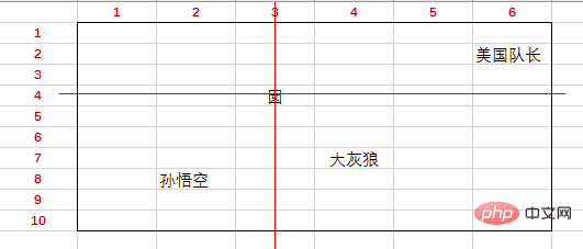
So the formula: =INDEX(B2:G11,4,3) can get "囡".

2. Basic usage of INDEX function
1. Extract values from a single row or column: only one coordinate value is required
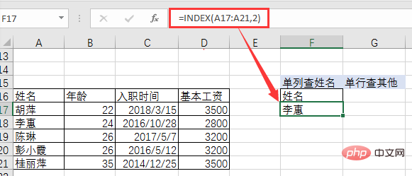
If the given area is a single row or column, then the coordinates do not need two numbers, only one.
For example, we now need to get "Li Hui" from A17:A21 in F17.
Enter the formula: =INDEX(A17:A21,2).
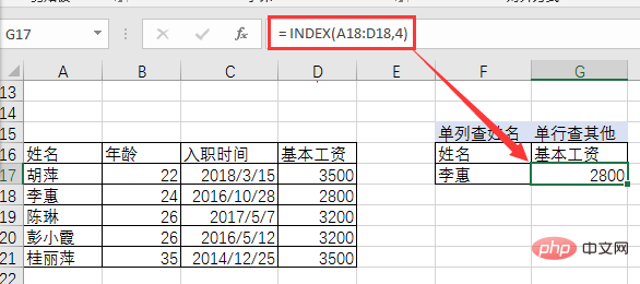
For another example, we need to obtain Li Hui’s basic salary from A18:D18 in G17.
Enter the formula: = INDEX(A18:D18,4).
2. Extract values from a multi-row and multi-column area: two coordinate values in rows and columns are required
This point will not be listed. . This is how you look for the word "囡" in the front.
As can be seen from the above example, INDEX returns a value through coordinates, like a precision-guided missile, hitting where it points (returning where). However, purely manual coordinate checking and then inputting the coordinates is not in line with "modernity". In actual operation, the data often consists of dozens of columns, dozens of rows or even tens of thousands of rows. At this time, it is too unrealistic for us to manually check the coordinates and enter the coordinates as needed. Therefore, INDEX needs assistants and a team to conquer the world.
3. Practical usage of INDEX

1. Group with assistants COLUMN and ROW: realize semi-automatic value search
(1) Grouping with COLUMN can continuously return multiple data of the same row
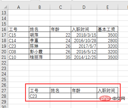
For example, we need to continuously obtain the name, age, and job number C23 from the table Entry Time.
In the data area A17:E21, the job number C23 is located in the 3rd row. The column numbers of name, age, and joining time are 2 and 3 respectively from left to right. ,4. We can use COLUMN (B1) to replace 2, 3, and 4 to achieve semi-automatic effects. The formula is as follows:
=INDEX($A17:$E21,3,COLUMN(B1))
Then pull right to fill in.

#The entry time obtained is a number, just change the format to a short date.
(2) Grouping with ROW can continuously return multiple data in the same column
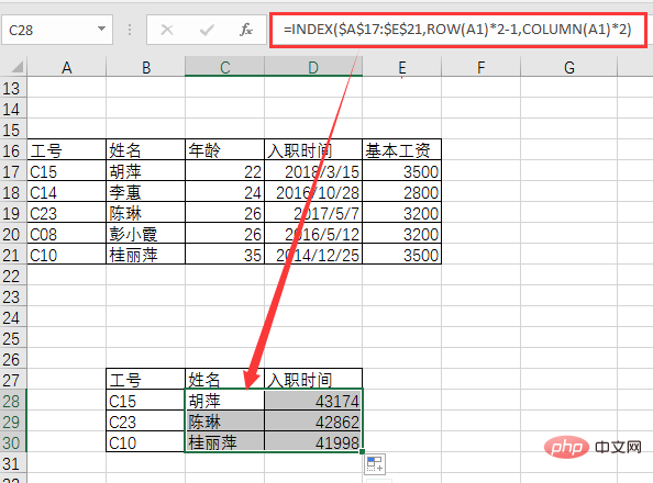
For example, below, we use the formula: =INDEX(A$17:E$21, ROW(A3),2) Drop down and fill in to get the names of three work numbers.
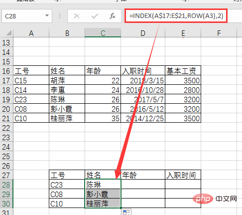
(3) Group together with COLUMN and ROW at the same time
For example, we can use the formula: =INDEX($A $17:$E$21,ROW(A3),COLUMN(B1))Pull right and drop down to fill in the name, age, and joining date of job numbers C23, C08, and C10.
By forming a group with COLUMN and ROW, a semi-automatic effect is achieved. As long as the values are continuous and regular, it can be achieved with INDEX ROW COLUMN.
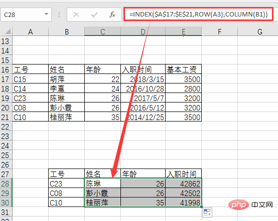
For example, we need to get values in alternate rows and columns to obtain the names and joining dates of job numbers C15, C23, and C10. The formula is:
=INDEX($A$17:$E$21,ROW(A1)*2-1,COLUMN(A1)*2)
Then right Just pull down to fill.
Semi-automatic is much easier than completely manual coordinate checking and inputting coordinates, but the reason why it is called semi-automatic is that it still requires manual work to find the rules of the data. If the data patterns of values are complex or irregular, we cannot be semi-automatic. At this time, you need to form a team with the big assistant MATCH to perform fully automatic work.
2. MATCH group with the assistant: realize fully automatic value search
(1) INDEX MATCH group
The following data search rules are messy. We don't need to find the rules ourselves, just leave everything to MATCH.
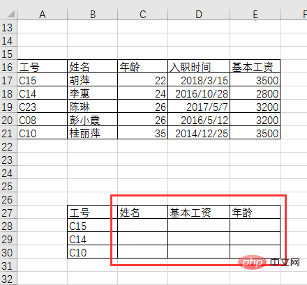
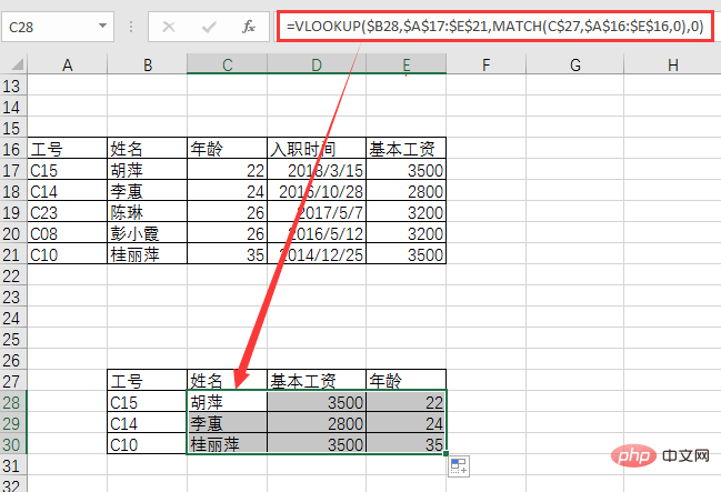
Enter the formula in C28:
=INDEX($A$17:$E$21,MATCH($B28,$A$17: $A$21,0),MATCH(C$27,$A$16:$E$16,0))
Then pull down to the right and fill in the formula.

Using the MATCH function to query row and column positions in a fixed area based on conditions completely replaces manual search for coordinates or data patterns, achieving full automation.
(2) The difference between INDEX MATCH and VLOOKUP MATCH
Input formula:
=VLOOKUP($B28,$ A$17:$E$21,MATCH(C$27,$A$16:$E$16,0),0)
Pull right and drop down to fill in.
In terms of formula length, VLOOKUP MATCH is simpler than INDEX MATCH. So why do we still need INDEX MATCH? The reason is that the INDEX function can find the data as long as it receives the row and column coordinate values. There is no difference between forward search and reverse search at all. VLOOKUP will not work. By default, it can only achieve forward search, that is, it can only search from left to right in the search area, but not from right to left. If VLOOKUP wants to implement a reverse search from right to left, it needs to use the IF function or CHOOSE function to construct a new search area.
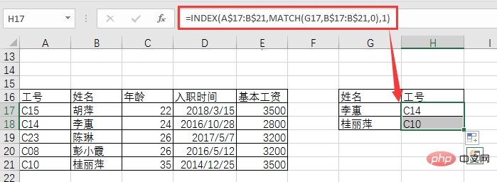
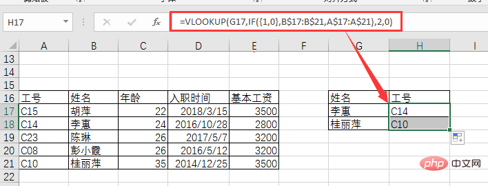
For example, we need to check the job number by name, as follows:
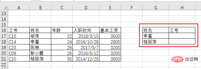
Use the INDEX MATCH combination to directly write the formula: =INDEX(A$17:B $21,MATCH(G17,B$17:B$21,0),1), and then pull down to
If you use VLOOKUP to search, because it is For reverse search, you need to use the IF function to reconstruct the search area. The formula becomes:
=VLOOKUP(G17,IF({1,0},B$17:B$21,A$17: A$21),2,0)
So, in comparison, when searching forward, both INDEX MATCH and VLOOKUP MATCH can be used, and VLOOKUP MATCH is relatively more efficient. Simple; when performing reverse search, INDEX MATCH is the simplest, especially when the reverse search area has three or four columns of data, INDEX MATCH is the best choice.
Okay, after answering the questions in Function Class 2, we continue to look at the practical grouping of INDEX.
3. Form a group with special guests SMALL and IF plus size assistants: realize one-to-many search
The formula format after grouping is =INDEX (Search area, SMALL(IF(),ROW()),MATCH())
For example, as shown in the animation below:
The formula is very long:
=INDEX($A$2:$D$21,SMALL(IF($C$2:$C$21=$F$2,ROW($1:$20), 99),ROW(A1)),MATCH(F$3,$A$1:$D$1,0))
If you apply the error-proof IFERROR function, it will be even longer:
=IFERROR(INDEX($A$2:$D$21,SMALL(IF($C$2:$C$21=$F$2,ROW($1:$20),99),ROW(A1)) ,MATCH(F$3,$A$1:$D$1,0)),"")
Such a combination formula, we often call it the snake oil formula, is mainly used for one-to-many search.
Ok, that’s all we’ve introduced about the practical usage of INDEX. The INDEX function has the advantage of using coordinates to accurately obtain values, but it lacks the function of automatically finding coordinates based on conditions. It is lame, so in actual combat it requires the assistance of an assistant to find coordinates. It's a precision-guided missile in function, and it's a Crip, a powerful Crip!
Related learning recommendations: excel tutorial
The above is the detailed content of Excel function learning: How to use the search function INDEX(). For more information, please follow other related articles on the PHP Chinese website!

Hot AI Tools

Undresser.AI Undress
AI-powered app for creating realistic nude photos

AI Clothes Remover
Online AI tool for removing clothes from photos.

Undress AI Tool
Undress images for free

Clothoff.io
AI clothes remover

AI Hentai Generator
Generate AI Hentai for free.

Hot Article
Hot Tools

Notepad++7.3.1
Easy-to-use and free code editor

SublimeText3 Chinese version
Chinese version, very easy to use

Zend Studio 13.0.1
Powerful PHP integrated development environment

Dreamweaver CS6
Visual web development tools

SublimeText3 Mac version
God-level code editing software (SublimeText3)
Hot Topics
 1385
1385
 52
52

 What should I do if the frame line disappears when printing in Excel?
Mar 21, 2024 am 09:50 AM
What should I do if the frame line disappears when printing in Excel?
Mar 21, 2024 am 09:50 AM
If when opening a file that needs to be printed, we will find that the table frame line has disappeared for some reason in the print preview. When encountering such a situation, we must deal with it in time. If this also appears in your print file If you have questions like this, then join the editor to learn the following course: What should I do if the frame line disappears when printing a table in Excel? 1. Open a file that needs to be printed, as shown in the figure below. 2. Select all required content areas, as shown in the figure below. 3. Right-click the mouse and select the "Format Cells" option, as shown in the figure below. 4. Click the “Border” option at the top of the window, as shown in the figure below. 5. Select the thin solid line pattern in the line style on the left, as shown in the figure below. 6. Select "Outer Border"
 How to filter more than 3 keywords at the same time in excel
Mar 21, 2024 pm 03:16 PM
How to filter more than 3 keywords at the same time in excel
Mar 21, 2024 pm 03:16 PM
Excel is often used to process data in daily office work, and it is often necessary to use the "filter" function. When we choose to perform "filtering" in Excel, we can only filter up to two conditions for the same column. So, do you know how to filter more than 3 keywords at the same time in Excel? Next, let me demonstrate it to you. The first method is to gradually add the conditions to the filter. If you want to filter out three qualifying details at the same time, you first need to filter out one of them step by step. At the beginning, you can first filter out employees with the surname "Wang" based on the conditions. Then click [OK], and then check [Add current selection to filter] in the filter results. The steps are as follows. Similarly, perform filtering separately again
 How to change excel table compatibility mode to normal mode
Mar 20, 2024 pm 08:01 PM
How to change excel table compatibility mode to normal mode
Mar 20, 2024 pm 08:01 PM
In our daily work and study, we copy Excel files from others, open them to add content or re-edit them, and then save them. Sometimes a compatibility check dialog box will appear, which is very troublesome. I don’t know Excel software. , can it be changed to normal mode? So below, the editor will bring you detailed steps to solve this problem, let us learn together. Finally, be sure to remember to save it. 1. Open a worksheet and display an additional compatibility mode in the name of the worksheet, as shown in the figure. 2. In this worksheet, after modifying the content and saving it, the dialog box of the compatibility checker always pops up. It is very troublesome to see this page, as shown in the figure. 3. Click the Office button, click Save As, and then
 How to type subscript in excel
Mar 20, 2024 am 11:31 AM
How to type subscript in excel
Mar 20, 2024 am 11:31 AM
eWe often use Excel to make some data tables and the like. Sometimes when entering parameter values, we need to superscript or subscript a certain number. For example, mathematical formulas are often used. So how do you type the subscript in Excel? ?Let’s take a look at the detailed steps: 1. Superscript method: 1. First, enter a3 (3 is superscript) in Excel. 2. Select the number "3", right-click and select "Format Cells". 3. Click "Superscript" and then "OK". 4. Look, the effect is like this. 2. Subscript method: 1. Similar to the superscript setting method, enter "ln310" (3 is the subscript) in the cell, select the number "3", right-click and select "Format Cells". 2. Check "Subscript" and click "OK"
 How to set superscript in excel
Mar 20, 2024 pm 04:30 PM
How to set superscript in excel
Mar 20, 2024 pm 04:30 PM
When processing data, sometimes we encounter data that contains various symbols such as multiples, temperatures, etc. Do you know how to set superscripts in Excel? When we use Excel to process data, if we do not set superscripts, it will make it more troublesome to enter a lot of our data. Today, the editor will bring you the specific setting method of excel superscript. 1. First, let us open the Microsoft Office Excel document on the desktop and select the text that needs to be modified into superscript, as shown in the figure. 2. Then, right-click and select the "Format Cells" option in the menu that appears after clicking, as shown in the figure. 3. Next, in the “Format Cells” dialog box that pops up automatically
 How to use the iif function in excel
Mar 20, 2024 pm 06:10 PM
How to use the iif function in excel
Mar 20, 2024 pm 06:10 PM
Most users use Excel to process table data. In fact, Excel also has a VBA program. Apart from experts, not many users have used this function. The iif function is often used when writing in VBA. It is actually the same as if The functions of the functions are similar. Let me introduce to you the usage of the iif function. There are iif functions in SQL statements and VBA code in Excel. The iif function is similar to the IF function in the excel worksheet. It performs true and false value judgment and returns different results based on the logically calculated true and false values. IF function usage is (condition, yes, no). IF statement and IIF function in VBA. The former IF statement is a control statement that can execute different statements according to conditions. The latter
 Where to set excel reading mode
Mar 21, 2024 am 08:40 AM
Where to set excel reading mode
Mar 21, 2024 am 08:40 AM
In the study of software, we are accustomed to using excel, not only because it is convenient, but also because it can meet a variety of formats needed in actual work, and excel is very flexible to use, and there is a mode that is convenient for reading. Today I brought For everyone: where to set the excel reading mode. 1. Turn on the computer, then open the Excel application and find the target data. 2. There are two ways to set the reading mode in Excel. The first one: In Excel, there are a large number of convenient processing methods distributed in the Excel layout. In the lower right corner of Excel, there is a shortcut to set the reading mode. Find the pattern of the cross mark and click it to enter the reading mode. There is a small three-dimensional mark on the right side of the cross mark.
 How to insert excel icons into PPT slides
Mar 26, 2024 pm 05:40 PM
How to insert excel icons into PPT slides
Mar 26, 2024 pm 05:40 PM
1. Open the PPT and turn the page to the page where you need to insert the excel icon. Click the Insert tab. 2. Click [Object]. 3. The following dialog box will pop up. 4. Click [Create from file] and click [Browse]. 5. Select the excel table to be inserted. 6. Click OK and the following page will pop up. 7. Check [Show as icon]. 8. Click OK.
