How to use DATEDIF() in Excel function learning

This article will introduce you to the DATEDIF function! The DATEDIF function can not only be used to calculate age, length of service, length of service salary, and project cycle, but can also be used to make birthday countdown reminders, project completion date countdown reminders, and so on. With it, you will never miss those important days again, whether it's a loved one's birthday, a project completion day, or your son or daughter's graduation day.

The DATEDIF function is different from the functions we usually see. As we all know, generally we only need to enter the first few letters of a function in EXCEL, and EXCEL will automatically pop up the function. However, after all the letters of the function have been entered, EXCEL still does not have any prompts. Some friends may wonder whether there is such a function. In fact, the DATEDIF function is a hidden function in EXCEL. It is not available in the help and insertion formulas, and can only be entered manually.

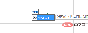
There is a prompt for non-hidden function input

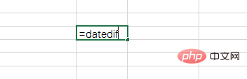
No prompt for hidden function input

The DATEDIF function can not only be used to calculate age, Length of service, seniority salary, project cycle, and can also be used as birthday countdown reminders, project completion date countdown reminders, etc. Let's get to know it below.

1. First introduction to DATEDIF

The DATEDIF function is used to calculate the difference between two dates and return the number of years, months and days between the two dates

Function structure: DATEDIF (start date, end date, return type)

1. Parameter explanation

1) Start date and end Date

Start date and end date are the two dates for which the difference needs to be calculated.

The input method of these two dates is as follows:

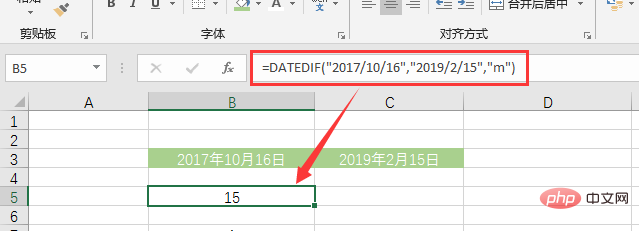
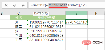
① You can directly enter the date with quotation marks, such as "2017/10/16". Note that the start date cannot be earlier than 1900, and the end date must be greater than the start date.

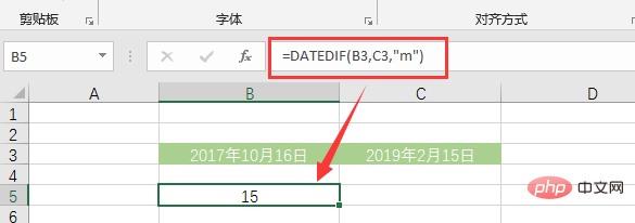
② You can also directly reference the date in the cell

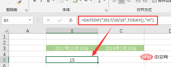
③ You can also use other functions to get it, such as TODAY () (Note: The day of the example is February 15, 2019)

##2) Return type

The return type is used for Set the type of settlement result. The return type is text, and double quotes are required when entering.

y: Returns the number of whole years between two dates (not counting if it is less than one year)

m: Returns the number of whole months (if it is less than one month)

d: Returns the number of days between two dates.

ym: Calculate the difference in whole months between two dates after omitting the difference in whole years. For example, if the two dates (2017-4-20, 2019-2-20) differ by 1 year and October, and the whole year is omitted and the difference is 1 year, the result of ym is October. For another example, if the two dates (2018-4-20, 2019-2-20) are 10 months apart, the result of ym is October.

yd: Calculate the difference in days between two dates after omitting the difference in whole years. For example, if the difference between two dates (2017-4-20, 2019-2-20) is 1 year and 306 days, and the whole year difference is omitted, the result of ym is 306 days.

md: Calculate the difference in days between two dates after omitting the difference in whole years and whole months. For example, if the difference between two dates (2017-4-20, 2019-2-25) is 1 year, 10 months and 5 days, and the difference of 1 year and 10 months is omitted, the result of md is 5 days.

2. Small chestnut

Give me a chestnut

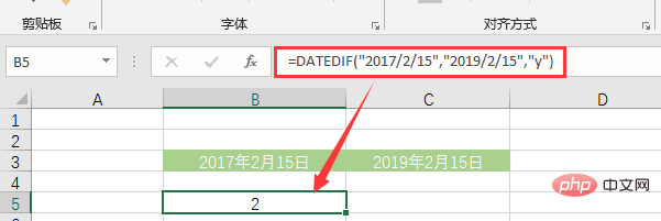
DATEDIF("2017/2/ 15","2019/2/15","y"), calculate the number of whole years difference between "2017/2/15" and "2019/2/15". The difference here is two complete years, so it equals 2.

DATEDIF("2017/1/6","2019/2/15","d"), calculate "2017/1/6" and "2019/ The number of days between 2/15" is equal to 770.

##DATEDIF("2017/1/6","2019/2/15","ym")

, calculate the difference between two dates The number of months apart from a full year. The actual difference between the two dates is 25 months, including 2 whole years (24 months), so the ym type return value is 25-24=1. 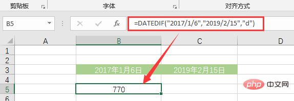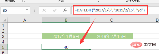<p><img src="/static/imghw/default1.png" data-src="https://img.php.cn/upload/article/000/000/024/aa1797dd147f6cfd77fe45e33627e0b4-10.png" class="lazy" style="max-width:90%" style="max-width:90%" alt="How to use DATEDIF() in Excel function learning" ></p> <p><code>DATEDIF("2017/1/6","2019/2/15","yd"), calculate the period between two dates excluding the whole year The number of days between. The actual difference between the two dates is 770 days, including 2 whole years (730 days), so the yd type return value is 770-730=40.

3. Use key points

1) Double quotes

to here, I believe that my friends already have a preliminary understanding of the DATEDIF function, and you can write a few formulas to practice. Please pay attention to the use of double quotation marks when writing formulas.

(1) If the 1st and 2nd parameters are to directly enter the date, the date must be in double quotes.

(2) The third parameter is text, so be sure to include double quotes.

2) Error type

If an error occurs in the DATEDIF function, there are usually three categories:

Error code	Error reason
NUM!	①The input value of the return type of the third parameter of the function is incorrect ②The first parameter is larger than the second parameter
#VALUE!	The start or end date refers to a cell format that is not a date format
#NAME?	①The function input is incorrect ②The text type data does not have double quotes

2. Practical application examples of DATEDIF function

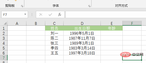
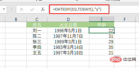
1. Calculate age based on date of birth

Given the date of birth of the following employees, Find their age this year.

No peeking at the answer~

Formula: =DATEDIF(D2,TODAY() ,"y")

##TODAY() function obtains the current date of the system. The example listed is the calculation result of 2019/2/15, and does not It must be consistent with the results obtained by my friends~ How about

? Isn't it very simple?

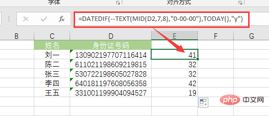
2. Calculate age based on ID number

The previous example already has the date of birth, so directly use the DATEDIF function to apply it The TODAY function can calculate age. If you only have an ID number, to calculate age, you need to extract the date of birth from the ID number and then calculate it. The formula is as follows:

① ② ③

Formula analysis:

①Use the MID function to extract the 8-digit number of the date of birth in the ID card number.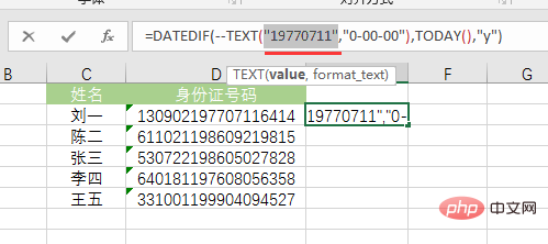

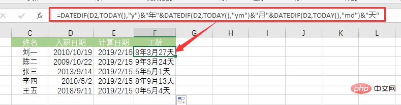
② Use the TEXT function to display these 8-digit numbers in the format of "0-00-00" to get text in a date format, and then add it before the TEXT function A negative-to-positive operation that converts text into a date.

③ Finally, use the date obtained above as the start date of the DATEDIF function, use TODAY() as the end date, and set the return type to "y" to calculate The number of whole years between two dates - age.

3. Calculate the employee’s length of service based on the date of joining (displayed in the form of year, month and day)

Use case 1 method of calculating age. If the time of employee joining is known, that is The employee's length of service in full years can be calculated. But if you need to calculate the detailed employee service length, such as how many years, months, and days, what should you do? The answer is as follows:

Although the formula is long, it is very easy to understand. First, use three DATEDIF functions to calculate the difference in years, months, and days between the two dates, and finally use the text connector "&" to connect to get the result.

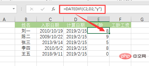
4. Calculate seniority wages

According to the seniority wage regulations promulgated by the state in 2019, employees who have worked continuously for one year are 50 yuan/month; employees who have been working continuously for two years are 100 yuan/month. Yuan/month; 150 Yuan/month for three consecutive years; 180 Yuan/month for four consecutive years, and so on, with a cumulative cap of ten years.

Are you confused? It’s okay, let’s go step by step, first calculate the length of service (calculated in full years).

Formula:

=DATEDIF(C2,D2,"y")

Then, come to our highlight, calculate the length of service salary.

Here we use the IF function and the MIN function.

According to the seniority wage regulations issued by the state in 2019, the salary for 1-3 years of service increases by 50 per year, and the salary for 4-10 years of service increases by 30 per year. We can use the IF function to judge separately.

First determine whether the seniority E2 is less than 4. If it is less than 4, it means that the employee's seniority salary is increased by 50 every year, and the result of "

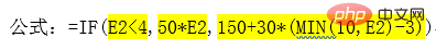
" is returned; if the seniority E2 is not less than 4, the seniority salary is 150 On the basis of increasing by 30 every year, the result of "" is returned.

Because the seniority salary can only be accumulated for ten years, and the seniority salary for more than ten years is consistent with the seniority salary for ten years, so we use the MIN function to return the minimum value between 10 and E2 as the seniority.

5. Make employee birthday reminder

The following is an employee information table. We want to make a birthday reminder to remind an employee 7 days in advance that his birthday is coming.

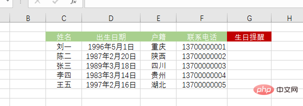
Tips: Use it in combination with the IF function, think about it~

                                                                                                                                                                                                     through

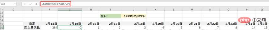
We usually calculate the number of days until the birthday by subtracting today's date from the upcoming birthday date. This formula is different from what we are used to. It calculates by subtracting the date of birth from today's date, and also reduces the date of birth by 7 days.

Why can this be done?

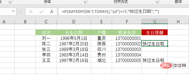
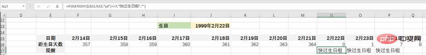
First, let’s take a look at the number of days between the current date and the date of birth under the yd return type. The following table takes the birth date of February 22, 1999 as an example, showing the number of days from yesterday, today, tomorrow, the day after tomorrow, etc. to the birth date.

N16 cell formula = DATEDIF($J$13,N15,"yd"), $J$13 represents the date of birth, and N15 represents a different current date.

Obviously, the interval on the birthday is 0; if it is less than the birthday date, the closer the date is to the birthday, the larger the interval is, the closer it is to 365; if it is greater than the birthday date, the closer the date is to the birthday, the smaller the interval is. Approaching 0.

Secondly, in this case, directly apply the IF function to give a birthday reminder formula based on whether the interval is less than or equal to 7 =IF(DATEDIF($J$13,N15,"yd") Birthday is coming soon La","") cannot realize the reminder 7 days in advance. On the contrary, it can only realize the reminder on the birthday and 7 days after the birthday, as follows:

Finally, what? Can I be reminded 7 days in advance? There are two methods. The first is to try to make the interval days 0-7 appear 7 days in advance. At this time, either reduce the start date by 7 days ($J$13-7), or change the end date Add 7 days (N15 7), as follows:

The number of days after the start date is reduced by 7 days

Birthday reminder after the start date is reduced by 7 days

The second method is to modify the judgment condition to >=358. As follows:

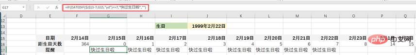
## Modification After judging the conditions, there will be no reminder on the birthday.

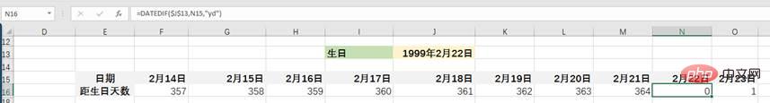
Ok, here, I believe everyone will understand the previous formula. On this basis, we can modify the formula to make the reminder more humane:

=IF(DATEDIF(D3-7,TODAY(),"yd")also"&7-DATEDIF(D3-7,TODAY(),"yd")&"It’s my birthday","")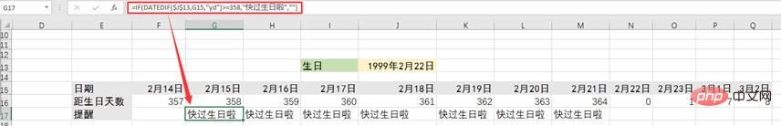

A few more words: If we use the usual idea of ​​subtracting the current date from the upcoming birthday date to calculate the number of days until the birthday, how should we write the birthday reminder formula? The answer is as follows:

=IF(DATEDIF(TODAY(),IF(TEXT(D3,"M月DD日")

月DD日"),YEAR(TODAY() 365),YEAR( TODAY()))&"year"&TEXT(D3,"M month DD day"),"yd")It's your birthday soon","")

(today(),"m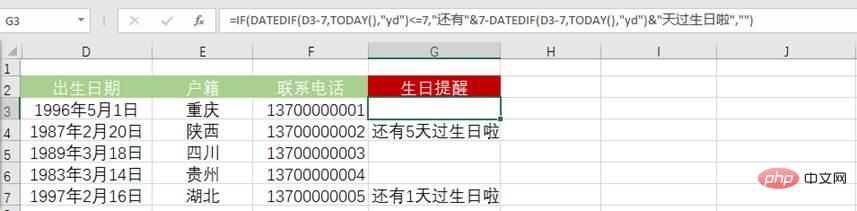

This is a very long formula!!!The long one is extracted from the upcoming birthday date.

IF(TEXT(D3) in the formula ,"M month DD day")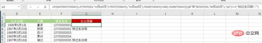month DD day"),YEAR(TODAY() 365),YEAR(TODAY()))&"Year"&TEXT(D3,"M month DD day") is used to obtain Upcoming birthday date. Meaning: If the number of months and days in the date of birth is less than the number of months and days today, it means that this year’s birthday has passed, and the new birthday date should be YEAR(TODAY() 365)&"Year"&TEXT(D3,"M month DD day "; On the contrary, it means that this year's birthday has not passed yet, and the birthday date should be YEAR(TODAY())&"年"&TEXT(D3,"M month DD day".

(today(),"m

YEAR(TODAY()) extracts this year's year and adds 365 to get next year's year.

TEXT(D3,"m month dd day") extracts the month and number in the date of birth.

At this point, the introduction of the DATEDIF function is complete. Whether it is calculating age, length of service, seniority wages, or giving birthday reminders, you can use DATEDIF. Of course, DATEDIF can also be used to calculate the project time, the number of days until completion, and provide a countdown reminder for completion. If you are doing personnel, payroll, or project management, then start practicing now!

Related learning recommendations: excel tutorial

The above is the detailed content of How to use DATEDIF() in Excel function learning. For more information, please follow other related articles on the PHP Chinese website!