

Excel function learning is one against ten SUBTOTAL functions!


Newbies always like to complain, "Excel has too many functions and I can't remember them. Is there a function that can summarize the functions of many functions?" I'll be honest with you. Say, there really is! The biggest function of the function we are going to talk about today is that it can replace 11 functions. In addition, it can also change the final calculation result based on different filtering results! How about it? Doesn’t it just sound awesome? Without further ado, let’s take a look with the editor!
Ignore the filtered row summation
"Teacher Miao, I encountered a problem", Xiaobai came to me as soon as she got to work, she Said: "I have a table of totals. I don't want to print the content of certain people when printing, so I hide them with filters. However, the summing area must be changed every time I sum, which is always troublesome."
I said: "That's easy, just change the summation function. Don't use SUM, try SUBTOTAL."
Xiaobai: "What kind of function is this? I've never used it before."
I said: "This function is much more powerful than the SUM function. It can handle several summation scenarios!"
Xiaobai: "It's so powerful, then you have to teach me."
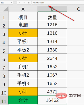
"Then let me tell you in detail~ First, let's solve the problem with your form." After saying that, I opened her form, as shown in the picture.
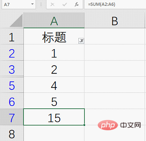
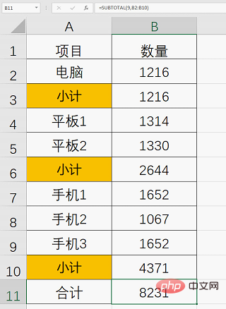
"Now, your table uses the SUM function for summation. Let's replace it with the SUBTOTAL function. You can take a look again." After that, I entered the formula in cell A7.
=SUBTOTAL(9,A2:A6)
"It's really changed!" Then Xiaobai filtered some more In other fields, she found that she could get the results she wanted, and she was very happy. But then she discovered the New World, "Then what does this 9 mean?"
Me: "This 9 means to ignore the unfiltered data and only sum the filtered results."
Xiaobai: "Listen to what you said, are there other numbers that represent other meanings?"
Me: "Of course, then I will tell you about the meanings of other numbers. !"
Ignore hidden row summation
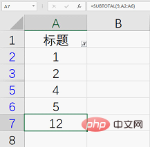
We sometimes encounter this situation. There is a column of numbers and we need to hide several different numbers. The data to perform operations on. If you use SUM directly, you cannot get the correct results, as shown in the figure.
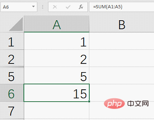
Even if you use the parameter "9" of the SUBTOTAL function you just learned, it cannot be achieved, as shown in the figure.
At this time we have to consider changing a parameter.
The following parameter is "109", come on!

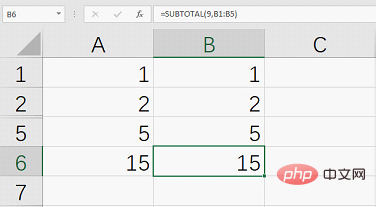
Formula: =SUBTOTAL(109,A1:A5)
As shown in the figure below, change the first parameter of the SUBTOTAL function to After it is "109", you can easily get the summation result after ignoring the hidden rows! as the picture shows.
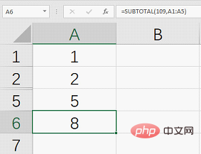
The function of parameter "109" is to sum the visible values. It can sum the hidden data or the filtered data. The parameter "9" can only be used in filtered rows and has no effect on hidden rows.
Application of other parameters of SUBTOTAL
SUBTOTAL is not limited to the field of summation, average, maximum, standard deviation, and variance are all You can find it, just change its first parameter. For example, now we want to count the maximum value of ignored hidden rows, as shown in Figure 6.
Formula: =SUBTOTAL(104,A1:A5)
## 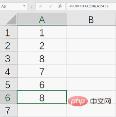
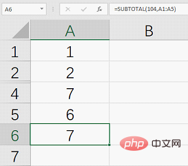
##After hiding the maximum value "8", the currently visible maximum value "7" is directly obtained in cell A6.
Then why is it 104? In fact, there is a set of number representation rules in the SUBTOTAL function. Today we will talk about the other parameters, including 11 functions such as average, maximum, minimum, standard deviation, and variance. Some are commonly used and some are not commonly used. You can choose based on your own needs. Below is a comparison table of 11 parameters.
Ignore filtered values when calculating |
Ignore hidden rows and filtered values when calculating |
Function |
Corresponding function |
| ##1 | 101 | AVERAGE | AVERAGE |
| 102 | Count the number of cells containing numbers | COUNT | |
| 103 | Calculate the number of non-empty cells | COUNTA | |
| ##104 | Maximum | MAX | |
| 105 | Minimum value | MIN |
|
6 |
106 |
Multiplication |
PRODUCT |
| ##7 | ##107Calculate sample standard deviation | STDEV | |
| 108 | Calculate population standard deviation | STDEVP | |
| 109 | SUM | SUM | |
##110 |
Calculate sample variance |
VAR |
11 |
111 |
Calculate population variance |
VARP |
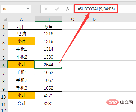
##Expansion Part 1: Only statistical classification and summary
When we are making tabulations, we often encounter such a summary situation, sub-summarizing in the same table, as shown in the figure shown.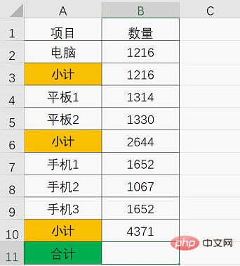
Expansion Part 2: Uninterrupted Serial Number
"After we understand the characteristics of the SUBTOTAL function, You can use it to do something, such as numbering a list.""What, can't the list number just be pulled with the mouse?""It's different~my number , but it’s automatic! Whether you delete rows or hide rows, the numbers can be rearranged automatically!”“It’s so magical, then I have to learn it hard.”In fact, it is very Simple, suppose I have a list, and the serial number column is currently empty, as shown in the picture.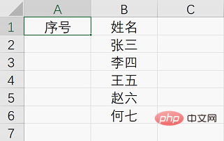
=SUBTOTAL(103,B$2:B2), then drop down to fill in, and you will get what we want serial number. as the picture shows.
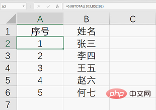
=SUBTOTAL(103,B$2:B2)
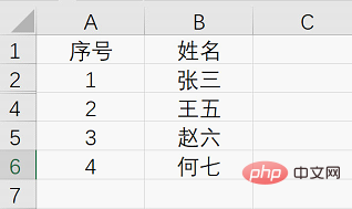
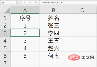
- 103: Looking at the above parameter comparison table, we can see that the function of 103 is to ignore hidden rows and filtered values, and count the number of non-empty cells.
- B$2:B2: The area in cell A2 is B$2:B2. The purpose is to count the number of non-empty cells in the B2:B2 area, and the result is 1. After the formula is pulled down, the area in cell A3 becomes B$2:B3, then the number of counted non-empty cells becomes two, and the result obtained is 2. as the picture shows.
The above is the detailed content of Excel function learning is one against ten SUBTOTAL functions!. For more information, please follow other related articles on the PHP Chinese website!

Hot AI Tools

Undresser.AI Undress
AI-powered app for creating realistic nude photos

AI Clothes Remover
Online AI tool for removing clothes from photos.

Undress AI Tool
Undress images for free

Clothoff.io
AI clothes remover

Video Face Swap
Swap faces in any video effortlessly with our completely free AI face swap tool!

Hot Article
Hot Tools

Notepad++7.3.1
Easy-to-use and free code editor

SublimeText3 Chinese version
Chinese version, very easy to use

Zend Studio 13.0.1
Powerful PHP integrated development environment

Dreamweaver CS6
Visual web development tools

SublimeText3 Mac version
God-level code editing software (SublimeText3)
Hot Topics
 1386
1386
 52
52

 What should I do if the frame line disappears when printing in Excel?
Mar 21, 2024 am 09:50 AM
What should I do if the frame line disappears when printing in Excel?
Mar 21, 2024 am 09:50 AM
If when opening a file that needs to be printed, we will find that the table frame line has disappeared for some reason in the print preview. When encountering such a situation, we must deal with it in time. If this also appears in your print file If you have questions like this, then join the editor to learn the following course: What should I do if the frame line disappears when printing a table in Excel? 1. Open a file that needs to be printed, as shown in the figure below. 2. Select all required content areas, as shown in the figure below. 3. Right-click the mouse and select the "Format Cells" option, as shown in the figure below. 4. Click the “Border” option at the top of the window, as shown in the figure below. 5. Select the thin solid line pattern in the line style on the left, as shown in the figure below. 6. Select "Outer Border"
 How to filter more than 3 keywords at the same time in excel
Mar 21, 2024 pm 03:16 PM
How to filter more than 3 keywords at the same time in excel
Mar 21, 2024 pm 03:16 PM
Excel is often used to process data in daily office work, and it is often necessary to use the "filter" function. When we choose to perform "filtering" in Excel, we can only filter up to two conditions for the same column. So, do you know how to filter more than 3 keywords at the same time in Excel? Next, let me demonstrate it to you. The first method is to gradually add the conditions to the filter. If you want to filter out three qualifying details at the same time, you first need to filter out one of them step by step. At the beginning, you can first filter out employees with the surname "Wang" based on the conditions. Then click [OK], and then check [Add current selection to filter] in the filter results. The steps are as follows. Similarly, perform filtering separately again
 How to change excel table compatibility mode to normal mode
Mar 20, 2024 pm 08:01 PM
How to change excel table compatibility mode to normal mode
Mar 20, 2024 pm 08:01 PM
In our daily work and study, we copy Excel files from others, open them to add content or re-edit them, and then save them. Sometimes a compatibility check dialog box will appear, which is very troublesome. I don’t know Excel software. , can it be changed to normal mode? So below, the editor will bring you detailed steps to solve this problem, let us learn together. Finally, be sure to remember to save it. 1. Open a worksheet and display an additional compatibility mode in the name of the worksheet, as shown in the figure. 2. In this worksheet, after modifying the content and saving it, the dialog box of the compatibility checker always pops up. It is very troublesome to see this page, as shown in the figure. 3. Click the Office button, click Save As, and then
 How to type subscript in excel
Mar 20, 2024 am 11:31 AM
How to type subscript in excel
Mar 20, 2024 am 11:31 AM
eWe often use Excel to make some data tables and the like. Sometimes when entering parameter values, we need to superscript or subscript a certain number. For example, mathematical formulas are often used. So how do you type the subscript in Excel? ?Let’s take a look at the detailed steps: 1. Superscript method: 1. First, enter a3 (3 is superscript) in Excel. 2. Select the number "3", right-click and select "Format Cells". 3. Click "Superscript" and then "OK". 4. Look, the effect is like this. 2. Subscript method: 1. Similar to the superscript setting method, enter "ln310" (3 is the subscript) in the cell, select the number "3", right-click and select "Format Cells". 2. Check "Subscript" and click "OK"
 How to set superscript in excel
Mar 20, 2024 pm 04:30 PM
How to set superscript in excel
Mar 20, 2024 pm 04:30 PM
When processing data, sometimes we encounter data that contains various symbols such as multiples, temperatures, etc. Do you know how to set superscripts in Excel? When we use Excel to process data, if we do not set superscripts, it will make it more troublesome to enter a lot of our data. Today, the editor will bring you the specific setting method of excel superscript. 1. First, let us open the Microsoft Office Excel document on the desktop and select the text that needs to be modified into superscript, as shown in the figure. 2. Then, right-click and select the "Format Cells" option in the menu that appears after clicking, as shown in the figure. 3. Next, in the “Format Cells” dialog box that pops up automatically
 How to use the iif function in excel
Mar 20, 2024 pm 06:10 PM
How to use the iif function in excel
Mar 20, 2024 pm 06:10 PM
Most users use Excel to process table data. In fact, Excel also has a VBA program. Apart from experts, not many users have used this function. The iif function is often used when writing in VBA. It is actually the same as if The functions of the functions are similar. Let me introduce to you the usage of the iif function. There are iif functions in SQL statements and VBA code in Excel. The iif function is similar to the IF function in the excel worksheet. It performs true and false value judgment and returns different results based on the logically calculated true and false values. IF function usage is (condition, yes, no). IF statement and IIF function in VBA. The former IF statement is a control statement that can execute different statements according to conditions. The latter
 Where to set excel reading mode
Mar 21, 2024 am 08:40 AM
Where to set excel reading mode
Mar 21, 2024 am 08:40 AM
In the study of software, we are accustomed to using excel, not only because it is convenient, but also because it can meet a variety of formats needed in actual work, and excel is very flexible to use, and there is a mode that is convenient for reading. Today I brought For everyone: where to set the excel reading mode. 1. Turn on the computer, then open the Excel application and find the target data. 2. There are two ways to set the reading mode in Excel. The first one: In Excel, there are a large number of convenient processing methods distributed in the Excel layout. In the lower right corner of Excel, there is a shortcut to set the reading mode. Find the pattern of the cross mark and click it to enter the reading mode. There is a small three-dimensional mark on the right side of the cross mark.
 How to insert excel icons into PPT slides
Mar 26, 2024 pm 05:40 PM
How to insert excel icons into PPT slides
Mar 26, 2024 pm 05:40 PM
1. Open the PPT and turn the page to the page where you need to insert the excel icon. Click the Insert tab. 2. Click [Object]. 3. The following dialog box will pop up. 4. Click [Create from file] and click [Browse]. 5. Select the excel table to be inserted. 6. Click OK and the following page will pop up. 7. Check [Show as icon]. 8. Click OK.
