Excel function learning: the dark horse in the query world - MAX()!

Isn’t MAX a function that finds the maximum value? When did you become the “dark horse in the query world”? Did VLOOKUP even feel defeated? The following article will give you an in-depth understanding of MAX's query function. I hope it will be helpful to you!

Everyone knows that VLOOKUP can match the data we need according to the given content. Because of this, it has a great reputation in the function community. But for the three examples I want to share today, if you use VLOOKUP to match the data, it will be a bit troublesome (interested friends can try it yourself). Just when VLOOKUP was having a headache, the MAX function solved all three problems with just one routine without saying a word.

Some friends may be curious, isn't MAX a function that finds the maximum value? How can it solve the problem that VLOOKUP can't solve? And what is this routine? Let’s take a look below to understand...

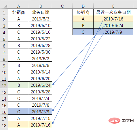
Example 1: Find the latest business date of each dealer in the business details

In order to facilitate understanding of the problem, the data source only retains two columns of data: dealer and business date. Now we need to get the date of the latest business for each dealer. (Tip: The business dates in the data source are arranged in ascending order.)

I don’t know how to use VLOOKUP to solve the problem? The routine used by MAX is as follows:

=MAX(($A$2:$A$18=D2)*$B$2:$B$18)

Please see the animation demonstration for the input method :

Note that after entering this formula, you must hold down the Ctrl and Shift keys at the same time and press Enter. Braces will automatically appear in the formula.

How to understand this formula is the question that everyone is most concerned about. In fact, the principle is very simple. First, make a comparison to see which data in column A is consistent with the supplier we need to judge, that is, $A$2: $A$18=$D2 is the function of this part. Select this part of the formula in the edit bar and press the F9 key to see the calculation results of the formula.

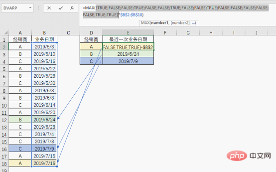
You can see that the result of the formula is a set of logical values. When the content of column A is consistent with the dealer to be matched, TRUE is obtained, otherwise FALSE is obtained.

The next step is to use this set of logical values ​​to multiply the business dates in column B (dates in Excel are essentially numbers). TRUE is the same as the number 1 when performing operations, and FALSE is performing operations. is the same as the number 0, so the calculation is like this.

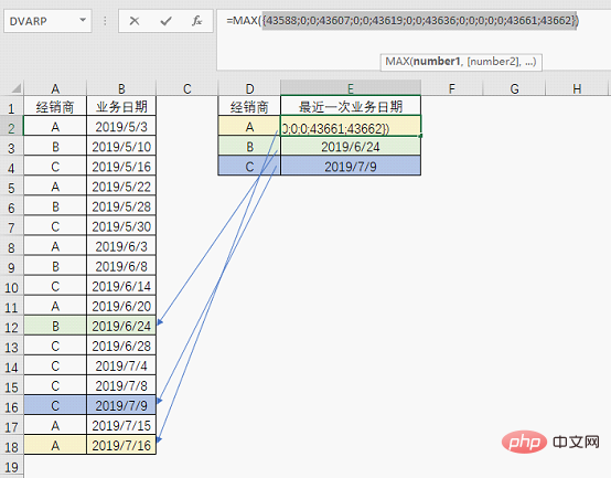
In the obtained set of numbers, 0 indicates the value returned when the corresponding dealer is not matched, and the numbers other than 0 indicate that the corresponding dealer is matched. The business date to be returned after business consultation. The largest value is the latest date, so MAX can easily get the final result.

If the result you produce is not a date but a number, it will be no problem to change the cell format to date format.

Example 2: Get the corresponding bonus according to the job number or name

Usually when performing data matching, a fixed condition is used Find. And in this example, our condition is one of the two.

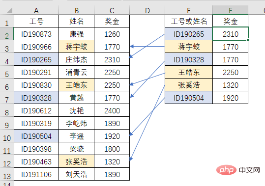
Regardless of the job number or name, you can get the corresponding bonus.

I don’t know how VLOOKUP can solve this problem? Anyway, MAX is still the same routine:

=MAX(($A$2:$B$13=E2)*$C$2:$C$13)

The formula entry method and principle will not be described in detail. It is exactly the same as Example 1. Let’s take a look at Example 3.

Example 3: Find the corresponding group code according to the name

Each group has four members, find the group it belongs to according to the name of the group member code.

If VLOOKUP still wants to struggle with the first two examples, this example can directly make VLOOKUP unable to find its way. MAX still follows the old routine:

=MAX(($B$2:$E$4=A7)*$A$2:$A$4)

##How about this routine of MAX function? Isn’t it very powerful?

To use this routine, you need to pay attention to the following two points:

1. The search result is a number;

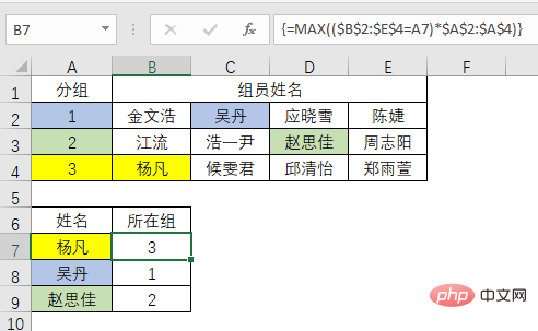
2. Note that the selection of the area for judging conditions and the area where the result is located must be accurate and locked.

Then the question comes, what if the result you want to find is not a number?

At this time, MAX alone cannot cope with it. IF or other functions are needed to meet the needs. We will introduce cases in this regard later.

Related learning recommendations: excel tutorial

The above is the detailed content of Excel function learning: the dark horse in the query world - MAX()!. For more information, please follow other related articles on the PHP Chinese website!