Practical Excel skills sharing: How to create two-level and three-level drop-down menus

When it comes to making drop-down menus, we all know that it can be achieved by directly using data verification in Excel, but second-level, third-level, or even higher-level drop-down menus may be a bit confusing. In fact, it is not difficult at all to use Excel to create a three-level drop-down menu. It is as simple as copying and pasting! Do not believe? Let’s read the article together and you will know!

Using data validation to create drop-down menus is familiar to most friends, but when it comes to second-level and third-level drop-down menus, you may not So familiar.

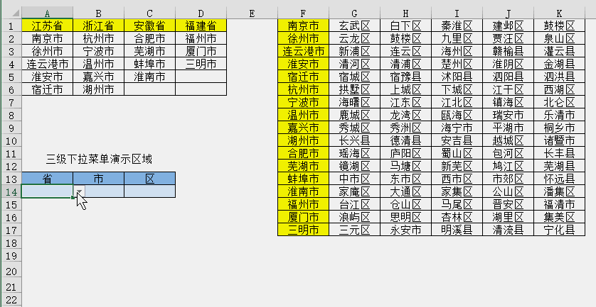
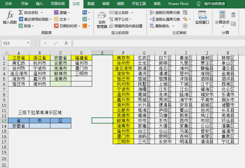
What are the second-level and third-level drop-down menus? For example, after selecting a province in a cell, only the city to which the province belongs can appear in the second cell option, and only the district to which the city belongs can appear in the third cell option. The effect is as shown in the figure.

It looks amazing. In fact, it is very easy to make such a multi-level drop-down menu. You only need to master two skills: defining names and data validation (data validity). ) can be achieved. Let’s take a look at the specific steps.

1. Create a first-level drop-down menu

Operation points:

[Quickly define name]Select the province where the name is located In the cell range "A1:D1", enter "Province" in the name box and press Enter to confirm;

[Set data verification] Select the cell where you want to set the first-level drop-down menu, open data verification, and set the sequence. Enter "=province" as the source, and a drop-down menu will be generated after confirmation. The operation steps are as shown in the animation.

Note: If "The specified named area does not exist" is prompted when setting data validation, it means that the definition of the name is incorrect.

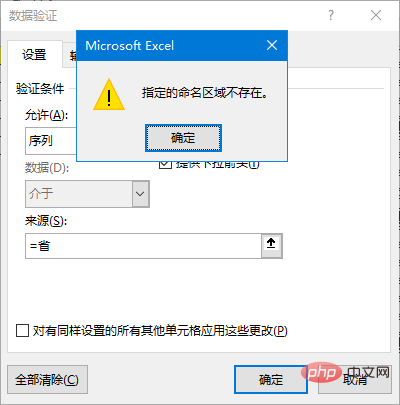
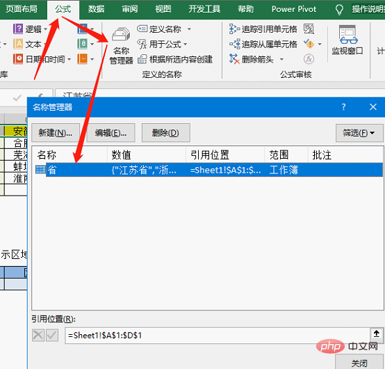
# Check whether the name is successfully defined by clicking "Formula-Name Manager".

After the above operations, the setting of the first-level drop-down menu is completed.

2. Create a secondary drop-down menu

Operation points:

[Batch definition name] Select the province and affiliation The cell range where the city is located, that is, "A1:D6", in the "Formulas" tab "Defined Name", click "Create from selected content" to batch define names, and only check the "First row" when creating ";

After completion, you can check it through the name manager. At this time, there will be several more names corresponding to the provinces.

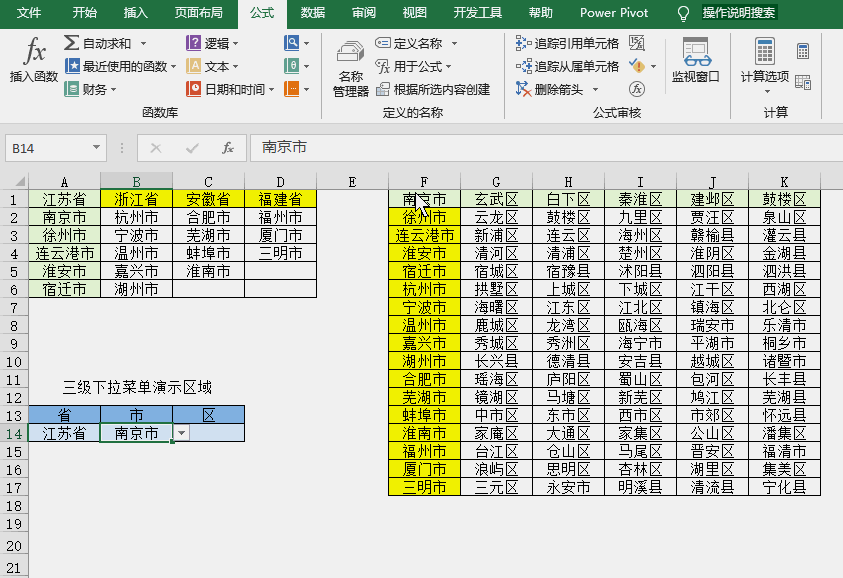
[Set data verification] Select the cell where you want to set the secondary drop-down menu, turn on the data verification, set the "sequence", enter "=INDIRECT(A14)" as the source, and after confirmation, the drop-down menu can be generated, and the operation The steps are shown in the animation.

In order to make it easier to set up the third-level menu later, we use a relative reference for A14 here.

Attention should be paid to this step: A14 in the formula needs to be modified according to the actual situation. The meaning of this formula is to use the cell data generated by the first-level menu as the basis for the effectiveness of the second-level menu.

After the above operations, the setting of the secondary drop-down menu is completed. You can verify the correctness of the options yourself.

About the INDIRECT function:

This function is a reference function. Simply speaking, it is quoted according to the specified address. In this example, A14 is a province name, and there is a set of corresponding cities in the name manager, as shown in the figure:

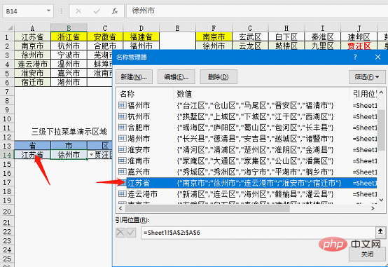
In this example, the function of the INDIRECT function is to get a set of names based on existing names. Corresponding data, if you need detailed tutorials on this function, you can leave a message to tell us.

3. Create a three-level drop-down menu

Operation points:

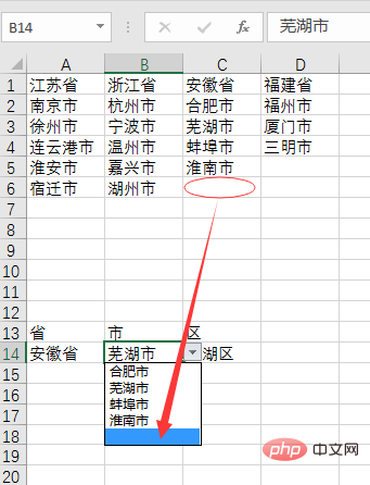
[Batch definition name ]Same as the previous step, select the cell range containing the city and district, that is, "F1:K17". Use the "Create from selected content" function to batch define names, and be careful to only check the "leftmost column" when creating;

[Copy Validity Settings] Copy the cell where the secondary drop-down menu is located, and when needed In the cell where the three-level drop-down menu is set, selectively paste "Verification" to complete the setting. The operation steps are as shown in the animation.

Because a relative reference is used in the validity formula of the cell where the secondary menu is located, just copy and paste cell B14 directly.

If you want to set the validity, the source should enter "=INDIRECT(B14)".

How about it, setting up the third-level menu is not that difficult.

Summary:

What I’m sharing today is just the most basic multi-level menu setting method. You need to pay attention to a few things.

1. When setting up a multi-level menu, the structure of the drop-down data source is very important. In this example, you can see the characteristics of the data source setting. As for whether the title should be in the first row or the leftmost column, it can be determined according to actual needs. Certainly.

2. The advantage of this setting method is that it is easy to master and easy to expand. According to the same method, it is not difficult to set up a fourth-level menu or even a fifth-level menu. But the disadvantages are also obvious. For example, when the number of options is different, blank options will appear in the drop-down box, and when the option content is increased, the name range needs to be modified, which is not very smart.

3. The core of setting up a multi-level menu is the usage of the INDIRECT function. If you want to make the drop-down menu more intelligent, do not contain blank items and automatically adjust when the content increases, You need to combine functions such as OFFSET, MATCH and COUNTA to achieve this. This requires considerable ability to use formula functions. If you are interested, please leave a message and tell the editor, and I will write another tutorial on this issue in the future.

Related learning recommendations: excel tutorial

The above is the detailed content of Practical Excel skills sharing: How to create two-level and three-level drop-down menus. For more information, please follow other related articles on the PHP Chinese website!