
 Technology peripherals
AI
Comparison of hyperparameter optimization: grid search, random search and Bayesian optimization
Technology peripherals
AI
Comparison of hyperparameter optimization: grid search, random search and Bayesian optimization
Comparison of hyperparameter optimization: grid search, random search and Bayesian optimization

This article will introduce in detail the most common hyperparameter optimization methods used to improve machine learning results.
Translator| The solution is to add more training data. Additional data is often helpful (except in certain circumstances), but generating high-quality data can be very expensive. Hyperparameter optimization saves us time and resources by using existing data to get the best model performance.
As the name suggests, hyperparameter optimization is the process of determining the best combination of hyperparameters for a machine learning model to satisfy the optimization function (i.e., maximize the performance of the model given the data set under study). In other words, each model provides multiple tuning “buttons” of options that we can change until we achieve an optimal combination of hyperparameters for our model. Some examples of parameters that we can change during hyperparameter optimization can be the learning rate, the architecture of the neural network (e.g., the number of hidden layers), regularization, etc.
In this article, we will conceptually introduce the three most common hyperparameter optimization methods, namely grid search, random search and Bayesian optimization, and then implement them one by one.
I will provide a high-level comparison table at the beginning of the article for the reader’s reference, and then further explore, explain, and implement each item in the comparison table throughout the rest of the article.
Table 1: Comparison of hyperparameter optimization methods1. Grid search algorithm Grid search may be a super The simplest and most intuitive method of parameter optimization, which involves an exhaustive search for the best combination of hyperparameters in a defined search space. The "search space" in this context is the entire hyperparameters and the values of such hyperparameters considered during optimization. Let’s understand grid search better with an example.
Suppose we have a machine learning model with only three parameters. Each parameter can take the value provided in the table:
parameter_1 = [1 , 2, 3]
parameter_2 = [a, b, c]parameter_3 = [x, y, z]
We don’t know which combination of these parameters will optimize our Optimization function of the model (i.e. providing the best output for our machine learning model). In grid search, we simply try every combination of these parameters, measure the model performance for each parameter, and simply choose the combination that yields the best performance! In this example, parameter 1 can take on 3 values (i.e. 1, 2, or 3), parameter 2 can take on 3 values (i.e. a, b, and c), and parameter 3 can take on 3 values (i.e. x, y, and z). In other words, there are 3*3*3=27 combinations in total. The grid search in this example will involve 27 rounds of evaluating the performance of the machine learning model to find the best performing combination.
As you can see, this method is very simple (similar to a trial and error task), but it also has some limitations. Let's summarize the advantages and disadvantages of this method.
Among them, the advantages include:
- Costly in large and/or complex models with a large number of hyperparameters (because all combinations must be tried and evaluated)
- No memory - no learning from the past Learning by Observation
- If the search space is too large, you may not be able to find the best combination. My suggestion is that if you have a simple model with a small search space, use grid search; otherwise, it is recommended to continue to Read on to find solutions better suited to larger search spaces. Now, let’s implement grid search using a real example.
- 1.1. Grid search algorithm implementation
- In order to implement grid search, we will use the Iris data set in scikit-learn to create a random forest classification model. This data set includes 3 different iris petal and sepal lengths and will be used for this classification exercise. In this paper, model development is secondary as the goal is to compare the performance of various hyperparameter optimization strategies. I encourage you to focus on the model evaluation results and the time required for each hyperparameter optimization method to reach the selected set of hyperparameters. I will describe the results of the run and then provide a summary comparison table for the three methods used in this article.
The search space including all hyperparameter values is defined as follows:
search_space = {'n_estimators': [10, 100, 500, 1000],
'max_depth' : [2, 10, 25, 50, 100],'min_samples_split': [2, 5, 10],
'min_samples_leaf': [1, 5, 10]}The above search space consists of a total combination of 4*5*3*3=180 hyperparameters. We will use grid search to find the combination that optimizes the objective function as follows:# Import libraries
from sklearn.model_selection import GridSearchCV
from sklearn.datasets import load_iris
from sklearn.ensemble import RandomForestClassifier
from sklearn.model_selection import cross_val_score
import time
# Load Iris data set
iris = load_iris()
X, y = iris.data, iris.target
#Define hyperparameter search space
search_space = {'n_estimators': [10, 100, 500, 1000],
'max_depth': [2, 10, 25, 50, 100],
'min_samples_split': [2, 5, 10 ],
'min_samples_leaf': [1, 5, 10]}
#Define Random Forest Classifier
clf = RandomForestClassifier(random_state=1234)
# Generate optimizer object
optimizer = GridSearchCV(clf, search_space, cv=5, scoring='accuracy')
#Storage the starting time for calculating the total time
start_time = time.time()
#Optimizer on fitting data
optimizer.fit(X, y)
# Store the end time so that it can be used to calculate the total time consuming
end_time = time.time ()
# Print the best hyperparameter set and corresponding score
print(f"selected hyperparameters:")
print(optimizer.best_params_)
print("")
print(f"best_score: {optimizer.best_score_}")
print(f"elapsed_time: {round(end_time-start_time, 1)}")
The output of the above code is as follows :
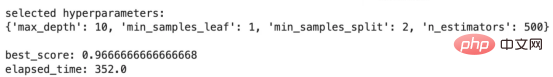
#Here we can see the hyperparameter values selected using grid search. Among them, best_score describes the evaluation results using the selected set of hyperparameters, and elapsed_time describes the time it took my local laptop to execute this hyperparameter optimization strategy. As you proceed to the next method, keep the evaluation results and elapsed time in mind for comparison. Now, let's get into the discussion of random search.
2. Random search algorithm
As the name suggests, random search is the process of randomly sampling hyperparameters from a defined search space. Unlike grid search, random search only selects a random subset of hyperparameter values for a predefined number of iterations (depending on available resources such as time, budget, goals, etc.) and computes the machine learning model for each hyperparameter performance, and then choose the best hyperparameter values.
Based on the above approach, you can imagine that random search is less expensive than a full grid search, but still has its own advantages and disadvantages, as follows:
Advantages:
- Easy to understand and implement
- Easy to parallelize
- Suitable for both discrete and continuous spaces
- Compared to grids Cheaper search
- More likely to converge to optimal than grid search with the same number of attempts Disadvantages:
- No memory – does not learn from past observations
- Considering random selection, important hyperparameter values may be missed
In the next method, we will solve the "memoryless" problem of grid and random search through Bayesian optimization "shortcoming. But before discussing this method, let's implement random search.
2.1. Random search algorithm implementation
Using the following code snippet, we will implement random search hyperparameter optimization for the same problem described in the grid search implementation.
# Import library
from sklearn.model_selection import RandomizedSearchCV
from scipy.stats import randint
# Create a RandomizedSearchCV object
optimizer = RandomizedSearchCV( clf, param_distributinotallow=search_space,
n_iter=50, cv=5, scoring='accuracy',
random_state=1234)
# Store the start time to calculate the total running time
start_time = time.time()
# Fit the optimizer on the data
optimizer.fit(X, y)
# Store the end time to calculate the total Running time
end_time = time.time()
# Print the optimal hyperparameter set and corresponding score
print(f"selected hyperparameters:")
print(optimizer .best_params_)
print("")
print(f"best_score: {optimizer.best_score_}")
print(f"elapsed_time: {round(end_time-start_time, 1)}" )
The output results of the above code are as follows:
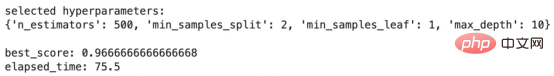
Random search results
Compared with the results of grid search, These results are very interesting. best_score remains the same, but elapsed_time decreases from 352.0 seconds to 75.5 seconds! How impressive! In other words, the random search algorithm managed to find a set of hyperparameters that performed the same as grid search in about 21% of the time required by grid search! However, the efficiency here is much higher.
Next, let’s move on to our next method, called Bayesian optimization, which learns from every attempt during the optimization process.
3. Bayesian Optimization
Bayesian optimization is a hyperparameter optimization method that uses a probabilistic model to "learn" from previous attempts and direct the search to the hyperparameters in the search space. The best combination to optimize the objective function of the machine learning model.
The Bayesian optimization method can be divided into 4 steps, which I will describe below. I encourage you to read through these steps to better understand the process, but there is no prerequisite knowledge required to use this method.
- Define a "prior", which is a probabilistic model evaluation of our beliefs about the most likely combination of hyperparameters to optimize the objective function at a certain point in time
- Evaluation Model of Hyperparameter Samples
- Use the knowledge gained in step 2 to update the probabilistic model in step 1 (what we call the “prior”) to understand the best hyperparameters that we believe optimize the objective function. Where are the possible combinations. Our updated belief is called the "posterior". In other words, the knowledge gained in step 2 helps us understand the search space better and takes us from the prior to the posterior, making the posterior our "latest" knowledge about the search space and objective function, as determined by step 2Provide information
- Repeat steps 2 and 3 until model performance converges, resources are exhausted, or other predefined metrics are met
If you are interested in learning more about Baye For detailed information on Si optimization, you can view the following post:
"Bayesian Optimization Algorithm in Machine Learning", the address is:
https://medium.com/@fmnobar/conceptual -overview-of-bayesian-optimization-for-parameter-tuning-in-machine-learning-a3b1b4b9339f.
Now, now that we understand how Bayesian optimization works, let’s look at its advantages and disadvantages.
Advantages:
- Learns from past observations and is therefore more efficient. In other words, it is expected to find a better set of hyperparameters in fewer iterations than memoryless methods that converge to the optimal given certain assumptions. Disadvantages:
- Difficult to parallelize
- Computationally intensive than grid and random search per iteration
- Prior and functions used in Bayesian optimization (e.g., The choice of the initial probability distribution for the acquisition function, etc.) can significantly affect the performance and its learning curve
- With the details out of the way, let’s implement Bayesian optimization and see the results.
3.1. Bayesian Optimization Algorithm Implementation
Similar to the previous section, we will use the following code snippet to implement Bayesian hyperparameters for the same problem described in Grid Search Implementation optimization.
# Import library
from skopt import BayesSearchCV
# Perform Bayesian optimization
optimizer = BayesSearchCV(estimator=RandomForestClassifier(),
search_spaces =search_space,
n_iter=10,
cv=5,
scoring='accuracy',
random_state=1234)
# Store the start time to calculate Total running time
start_time = time.time()
optimizer.fit(X, y)
# Store the end time to calculate the total running time
end_time = time.time()
# Print the best hyperparameter set and corresponding score
print(f"selected hyperparameters:")
print(optimizer.best_params_)
print("")
print(f"best_score: {optimizer.best_score_}")
print(f"elapsed_time: {round(end_time-start_time, 1)}")
The output results of the above code are as follows:
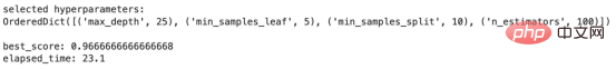 Bayesian optimization results
Another set of interesting results! The best_score is consistent with the results we obtained with grid and random search, but the result took only 23.1 seconds compared to 75.5 seconds for random search and 352.0 seconds for grid search! In other words, using Bayesian optimization takes approximately 93% less time than grid search. This is a huge productivity boost that becomes even more meaningful in larger, more complex models and search spaces.
Note that Bayesian optimization only used 10 iterations to obtain these results because it can learn from previous iterations (as opposed to random and grid search).
Result Comparison
The table below compares the results of the three methods discussed so far. The “Methodology” column describes the hyperparameter optimization method used. This is followed by the hyperparameters selected using each method. "Best Score" is the score obtained using a specific method, and then "Elapsed Time" represents how long it took for the optimization strategy to run on my local laptop. The last column, Gained Efficiency, assumes grid search as the baseline and then calculates the efficiency gained by each of the other two methods compared to grid search (using elapsed time). For example, since random search takes 75.5 seconds and grid search takes 352.0 seconds, the efficiency of random search relative to the grid search baseline is calculated as 1–75.5/352.0=78.5%.

Table 2 - Method Performance Comparison Table
Two main conclusions in the above comparison table:
- Efficiency: We can see how learning methods such as Bayesian optimization can find an optimized set of hyperparameters in less time.
- Parameter selection: There can be multiple correct answers. For example, the selected parameters for Bayesian optimization are different from those for grid and random search, although the evaluation metric (i.e. best_score) remains the same. This is even more important in larger, more complex environments.
Conclusion
In this article, we discussed what hyperparameter optimization is and introduced the three most common methods used for this optimization exercise. We then introduce each of these three methods in detail and implement them in a classification exercise. Finally, we compare the results of implementing the three methods. We find that methods such as Bayesian optimization learned from previous attempts can significantly improve efficiency, which can be an important factor in large complex models such as deep neural networks, where efficiency can be a determining factor.
Translator Introduction
Zhu Xianzhong, 51CTO community editor, 51CTO expert blogger, lecturer, computer teacher at a university in Weifang, and a veteran in the freelance programming industry.
Original title: Hyperparameter Optimization — Intro and Implementation of Grid Search, Random Search and Bayesian Optimization, author: Farzad Mahmoodinobar
The above is the detailed content of Comparison of hyperparameter optimization: grid search, random search and Bayesian optimization. For more information, please follow other related articles on the PHP Chinese website!

Hot AI Tools

Undresser.AI Undress
AI-powered app for creating realistic nude photos

AI Clothes Remover
Online AI tool for removing clothes from photos.

Undress AI Tool
Undress images for free

Clothoff.io
AI clothes remover

Video Face Swap
Swap faces in any video effortlessly with our completely free AI face swap tool!

Hot Article
Hot Tools

Notepad++7.3.1
Easy-to-use and free code editor

SublimeText3 Chinese version
Chinese version, very easy to use

Zend Studio 13.0.1
Powerful PHP integrated development environment

Dreamweaver CS6
Visual web development tools

SublimeText3 Mac version
God-level code editing software (SublimeText3)
Hot Topics
 1392
1392
 52
36
110
52
36
110

 Bytedance Cutting launches SVIP super membership: 499 yuan for continuous annual subscription, providing a variety of AI functions
Jun 28, 2024 am 03:51 AM
Bytedance Cutting launches SVIP super membership: 499 yuan for continuous annual subscription, providing a variety of AI functions
Jun 28, 2024 am 03:51 AM
This site reported on June 27 that Jianying is a video editing software developed by FaceMeng Technology, a subsidiary of ByteDance. It relies on the Douyin platform and basically produces short video content for users of the platform. It is compatible with iOS, Android, and Windows. , MacOS and other operating systems. Jianying officially announced the upgrade of its membership system and launched a new SVIP, which includes a variety of AI black technologies, such as intelligent translation, intelligent highlighting, intelligent packaging, digital human synthesis, etc. In terms of price, the monthly fee for clipping SVIP is 79 yuan, the annual fee is 599 yuan (note on this site: equivalent to 49.9 yuan per month), the continuous monthly subscription is 59 yuan per month, and the continuous annual subscription is 499 yuan per year (equivalent to 41.6 yuan per month) . In addition, the cut official also stated that in order to improve the user experience, those who have subscribed to the original VIP
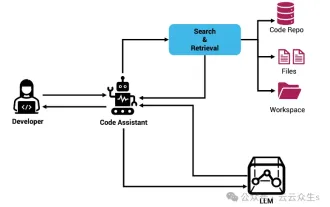 Context-augmented AI coding assistant using Rag and Sem-Rag
Jun 10, 2024 am 11:08 AM
Context-augmented AI coding assistant using Rag and Sem-Rag
Jun 10, 2024 am 11:08 AM
Improve developer productivity, efficiency, and accuracy by incorporating retrieval-enhanced generation and semantic memory into AI coding assistants. Translated from EnhancingAICodingAssistantswithContextUsingRAGandSEM-RAG, author JanakiramMSV. While basic AI programming assistants are naturally helpful, they often fail to provide the most relevant and correct code suggestions because they rely on a general understanding of the software language and the most common patterns of writing software. The code generated by these coding assistants is suitable for solving the problems they are responsible for solving, but often does not conform to the coding standards, conventions and styles of the individual teams. This often results in suggestions that need to be modified or refined in order for the code to be accepted into the application
 Can fine-tuning really allow LLM to learn new things: introducing new knowledge may make the model produce more hallucinations
Jun 11, 2024 pm 03:57 PM
Can fine-tuning really allow LLM to learn new things: introducing new knowledge may make the model produce more hallucinations
Jun 11, 2024 pm 03:57 PM
Large Language Models (LLMs) are trained on huge text databases, where they acquire large amounts of real-world knowledge. This knowledge is embedded into their parameters and can then be used when needed. The knowledge of these models is "reified" at the end of training. At the end of pre-training, the model actually stops learning. Align or fine-tune the model to learn how to leverage this knowledge and respond more naturally to user questions. But sometimes model knowledge is not enough, and although the model can access external content through RAG, it is considered beneficial to adapt the model to new domains through fine-tuning. This fine-tuning is performed using input from human annotators or other LLM creations, where the model encounters additional real-world knowledge and integrates it
 Seven Cool GenAI & LLM Technical Interview Questions
Jun 07, 2024 am 10:06 AM
Seven Cool GenAI & LLM Technical Interview Questions
Jun 07, 2024 am 10:06 AM
To learn more about AIGC, please visit: 51CTOAI.x Community https://www.51cto.com/aigc/Translator|Jingyan Reviewer|Chonglou is different from the traditional question bank that can be seen everywhere on the Internet. These questions It requires thinking outside the box. Large Language Models (LLMs) are increasingly important in the fields of data science, generative artificial intelligence (GenAI), and artificial intelligence. These complex algorithms enhance human skills and drive efficiency and innovation in many industries, becoming the key for companies to remain competitive. LLM has a wide range of applications. It can be used in fields such as natural language processing, text generation, speech recognition and recommendation systems. By learning from large amounts of data, LLM is able to generate text
 Five schools of machine learning you don't know about
Jun 05, 2024 pm 08:51 PM
Five schools of machine learning you don't know about
Jun 05, 2024 pm 08:51 PM
Machine learning is an important branch of artificial intelligence that gives computers the ability to learn from data and improve their capabilities without being explicitly programmed. Machine learning has a wide range of applications in various fields, from image recognition and natural language processing to recommendation systems and fraud detection, and it is changing the way we live. There are many different methods and theories in the field of machine learning, among which the five most influential methods are called the "Five Schools of Machine Learning". The five major schools are the symbolic school, the connectionist school, the evolutionary school, the Bayesian school and the analogy school. 1. Symbolism, also known as symbolism, emphasizes the use of symbols for logical reasoning and expression of knowledge. This school of thought believes that learning is a process of reverse deduction, through existing
 To provide a new scientific and complex question answering benchmark and evaluation system for large models, UNSW, Argonne, University of Chicago and other institutions jointly launched the SciQAG framework
Jul 25, 2024 am 06:42 AM
To provide a new scientific and complex question answering benchmark and evaluation system for large models, UNSW, Argonne, University of Chicago and other institutions jointly launched the SciQAG framework
Jul 25, 2024 am 06:42 AM
Editor |ScienceAI Question Answering (QA) data set plays a vital role in promoting natural language processing (NLP) research. High-quality QA data sets can not only be used to fine-tune models, but also effectively evaluate the capabilities of large language models (LLM), especially the ability to understand and reason about scientific knowledge. Although there are currently many scientific QA data sets covering medicine, chemistry, biology and other fields, these data sets still have some shortcomings. First, the data form is relatively simple, most of which are multiple-choice questions. They are easy to evaluate, but limit the model's answer selection range and cannot fully test the model's ability to answer scientific questions. In contrast, open-ended Q&A
 SOTA performance, Xiamen multi-modal protein-ligand affinity prediction AI method, combines molecular surface information for the first time
Jul 17, 2024 pm 06:37 PM
SOTA performance, Xiamen multi-modal protein-ligand affinity prediction AI method, combines molecular surface information for the first time
Jul 17, 2024 pm 06:37 PM
Editor | KX In the field of drug research and development, accurately and effectively predicting the binding affinity of proteins and ligands is crucial for drug screening and optimization. However, current studies do not take into account the important role of molecular surface information in protein-ligand interactions. Based on this, researchers from Xiamen University proposed a novel multi-modal feature extraction (MFE) framework, which for the first time combines information on protein surface, 3D structure and sequence, and uses a cross-attention mechanism to compare different modalities. feature alignment. Experimental results demonstrate that this method achieves state-of-the-art performance in predicting protein-ligand binding affinities. Furthermore, ablation studies demonstrate the effectiveness and necessity of protein surface information and multimodal feature alignment within this framework. Related research begins with "S
 SK Hynix will display new AI-related products on August 6: 12-layer HBM3E, 321-high NAND, etc.
Aug 01, 2024 pm 09:40 PM
SK Hynix will display new AI-related products on August 6: 12-layer HBM3E, 321-high NAND, etc.
Aug 01, 2024 pm 09:40 PM
According to news from this site on August 1, SK Hynix released a blog post today (August 1), announcing that it will attend the Global Semiconductor Memory Summit FMS2024 to be held in Santa Clara, California, USA from August 6 to 8, showcasing many new technologies. generation product. Introduction to the Future Memory and Storage Summit (FutureMemoryandStorage), formerly the Flash Memory Summit (FlashMemorySummit) mainly for NAND suppliers, in the context of increasing attention to artificial intelligence technology, this year was renamed the Future Memory and Storage Summit (FutureMemoryandStorage) to invite DRAM and storage vendors and many more players. New product SK hynix launched last year
