

How to use XGBoost and InluxDB for time series forecasting

XGBoost is a popular open source machine learning library that can be used to solve a variety of prediction problems. One needs to understand how to use it with InfluxDB for time series forecasting.
Translator | Li Rui
Reviewer | Sun Shujuan
XGBoost is an open source machine learning library that implements an optimized distributed gradient boosting algorithm. XGBoost uses parallel processing for fast performance, handles missing values well, performs well on small datasets, and prevents overfitting. All these advantages make XGBoost a popular solution for regression problems such as prediction.
Forecasting is mission-critical for various business goals such as predictive analytics, predictive maintenance, product planning, budgeting, etc. Many forecasting or forecasting problems involve time series data. This makes XGBoost an excellent partner for the open source time series database InfluxDB.
This tutorial will learn how to use XGBoost’s Python package to predict data from the InfluxDB time series database. You will also use the InfluxDB Python client library to query data from InfluxDB and convert the data to a Pandas DataFrame to make it easier to work with time series data before making predictions. Additionally, the advantages of XGBoost will be discussed in more detail.
1. Requirements
This tutorial is performed on a macOS system with Python 3 installed through Homebrew. It is recommended to set up additional tools such as virtualenv, pyenv or conda-env to simplify Python and client installation. Otherwise, its full requirements are as follows:
- influxdb-client=1.30.0
- pandas = 1.4.3
- xgboost>=1.7.3
- influxdb-client>=1.30.0
- pandas>=1.4.3
- matplotlib>=3.5.2
- sklearn>=1.1.1
This tutorial also assumes that you have a free tier InfluxDB cloud account and that you have created a bucket and a token. Think of a bucket as the database or the highest level of data organization in InfluxDB. In this tutorial, a bucket named NOAA will be created.
2. Decision trees, random forests and gradient enhancement
In order to understand what XGBoost is, you must understand decision trees, random forests and gradient enhancement. Decision trees are a supervised learning method consisting of a series of feature tests. Each node is a test, and all nodes are organized in a flowchart structure. Branches represent conditions that ultimately determine which leaf label or class label is assigned to the input data.

# Decision trees in machine learning are used to determine whether it will rain tomorrow. Edited to show the components of a decision tree: leaves, branches, and nodes.
The guiding principle behind decision trees, random forests, and gradient boosting is that multiple "weak learners" or classifiers work together to make strong predictions.
Random forest contains multiple decision trees. Each node in a decision tree is considered a weak learner, and each decision tree in a random forest is considered one of many weak learners in a random forest model. Typically, all data is randomly divided into subsets and passed through different decision trees.
Gradient boosting using decision trees and random forests is similar, but the way they are structured is different. Gradient boosted trees also contain decision tree forests, but these decision trees are additionally constructed and all the data is passed through the decision tree ensemble. Gradient boosting trees may consist of a set of classification trees or regression trees, with classification trees for discrete values (such as cats or dogs). Regression trees are used for continuous values (e.g. 0 to 100).
3. What is XGBoost?
Gradient boosting is a machine learning algorithm used for classification and prediction. XGBoost is just an extreme type of gradient boosting. At its extreme, gradient boosting can be performed more efficiently through the power of parallel processing. The image below from the XGBoost documentation illustrates how gradient boosting can be used to predict whether someone will like a video game.

#Two decision trees are used to decide whether someone is likely to like a video game. Add the leaf scores from both trees to determine which person is most likely to enjoy the video game.
Some advantages of XGBoost:
- Relatively easy to understand.
- Suitable for small, structured and regular data with few features.
Some disadvantages of XGBoost:
- Easy to overfitting and sensitive to outliers. It might be a good idea to use materialized views of time series data in XGBoost for forecasting.
- Performs poorly on sparse or unsupervised data.
4. Use XGBoost for time series prediction
The air sensor sample data set used here is provided by InfluxDB. This dataset contains temperature data from multiple sensors. A temperature forecast is being created for a single sensor with data like this:

Use the following Flux code to import the dataset and filter for a single time series. (Flux is the query language of InfluxDB)
import "join"
import "influxdata/influxdb/sample"
//dataset is regular time series at 10 second intervals
data = sample.data(set: "airSensor")
|> filter(fn: (r) => r._field == "temperature" and r.sensor_id == "TLM0100")
Random forest and gradient boosting can be used for time series forecasting, but they require converting the data to supervised learning. This means that the data must be moved forward in a sliding window approach or a slow-moving approach to convert the time series data into a supervised learning set. The data can also be prepared with Flux. Ideally, some autocorrelation analysis should be performed first to determine the best method to use. For the sake of brevity, the following Flux code will be used to move data at a regular interval.
import "join"
import "influxdata/influxdb/sample"
data = sample.data(set: "airSensor")
|> ; filter(fn: (r) => r._field == "temperature" and r.sensor_id == "TLM0100")
shiftedData = data
|> timeShift(duration : 10s, columns: ["_time"] )
join.time(left: data, right: shiftedData, as: (l, r) => ({l with data: l._value, shiftedData : r._value}))
|> drop(columns: ["_measurement", "_time", "_value", "sensor_id", "_field"])
Swipe left and right to see the complete code

If you want to add additional lag data to the model input, you can follow the following Flux logic instead.
import "experimental"
import "influxdata/influxdb/sample"
data = sample.data(set: "airSensor")
|> ; filter(fn: (r) => r._field == "temperature" and r.sensor_id == "TLM0100")
shiftedData1 = data
|> timeShift(duration: 10s, columns: ["_time"] )
|> set(key: "shift" , value: "1" )
shiftedData2 = data
|> timeShift(duration: 20s , columns: ["_time"] )
|> set(key: "shift" , value: "2" )
shiftedData3 = data
|> timeShift(duration: 30s , columns: ["_time"] )
|> set( key: "shift" , value: "3")
shiftedData4 = data
|> timeShift(duration: 40s , columns: ["_time"] )
|> set(key: "shift" , value: "4")
##union(tables: [shiftedData1, shiftedData2, shiftedData3, shiftedData4])
|> pivot(rowKey:["_time"], columnKey: ["shift"], valueColumn: "_value")
|> drop(columns: ["_measurement", "_time", "_value", "sensor_id", "_field"])
// remove the NaN values
|> limit(n:360)
|> tail(n: 356)

import pandas as pd
from numpy import asarray
from sklearn.metrics import mean_absolute_error
from xgboost import XGBRegressor
from matplotlib import pyplot
from influxdb_client import InfluxDBClient
from influxdb_client.client.write_api import SYNCHRONOUS
# query data with the Python InfluxDB Client Library and transform data into a supervised learning problem with Flux
client = InfluxDBClient(url="https://us-west-2-1.aws.cloud2.influxdata.com", token="NyP-HzFGkObUBI4Wwg6Rbd-_SdrTMtZzbFK921VkMQWp3bv_e9BhpBi6fCBr_0-6i0ev32_XWZcmkDPsearTWA==", org="0437f6d51b579000")
# write_api = client.write_api(write_optinotallow=SYNCHRONOUS)
query_api = client.query_api()
df = query_api.query_data_frame('import "join"'
'import "influxdata/influxdb/sample"'
'data = sample.data(set: "airSensor")'
'|> filter(fn: (r) => r._field == "temperature" and r.sensor_id == "TLM0100")'
'shiftedData = data'
'|> timeShift(duration: 10s , columns: ["_time"] )'
'join.time(left: data, right: shiftedData, as: (l, r) => ({l with data: l._value, shiftedData: r._value}))'
'|> drop(columns: ["_measurement", "_time", "_value", "sensor_id", "_field"])'
'|> yield(name: "converted to supervised learning dataset")'
)
df = df.drop(columns=['table', 'result'])
data = df.to_numpy()
# split a univariate dataset into train/test sets
def train_test_split(data, n_test):
return data[:-n_test:], data[-n_test:]
# fit an xgboost model and make a one step prediction
def xgboost_forecast(train, testX):
# transform list into array
train = asarray(train)
# split into input and output columns
trainX, trainy = train[:, :-1], train[:, -1]
# fit model
model = XGBRegressor(objective='reg:squarederror', n_estimators=1000)
model.fit(trainX, trainy)
# make a one-step prediction
yhat = model.predict(asarray([testX]))
return yhat[0]
# walk-forward validation for univariate data
def walk_forward_validation(data, n_test):
predictions = list()
# split dataset
train, test = train_test_split(data, n_test)
history = [x for x in train]
# step over each time-step in the test set
for i in range(len(test)):
# split test row into input and output columns
testX, testy = test[i, :-1], test[i, -1]
# fit model on history and make a prediction
yhat = xgboost_forecast(history, testX)
# store forecast in list of predictions
predictions.append(yhat)
# add actual observation to history for the next loop
history.append(test[i])
# summarize progress
print('>expected=%.1f, predicted=%.1f' % (testy, yhat))
# estimate prediction error
error = mean_absolute_error(test[:, -1], predictions)
return error, test[:, -1], predictions
# evaluate
mae, y, yhat = walk_forward_validation(data, 100)
print('MAE: %.3f' % mae)
# plot expected vs predicted
pyplot.plot(y, label='Expected')
pyplot.plot(yhat, label='Predicted')
pyplot.legend()
pyplot.show()
五、结论
希望这篇博文能够激励人们利用XGBoost和InfluxDB进行预测。为此建议查看相关的报告,其中包括如何使用本文描述的许多算法和InfluxDB来进行预测和执行异常检测的示例。
原文链接:https://www.infoworld.com/article/3682070/time-series-forecasting-with-xgboost-and-influxdb.html

The above is the detailed content of How to use XGBoost and InluxDB for time series forecasting. For more information, please follow other related articles on the PHP Chinese website!

Hot AI Tools

Undresser.AI Undress
AI-powered app for creating realistic nude photos

AI Clothes Remover
Online AI tool for removing clothes from photos.

Undress AI Tool
Undress images for free

Clothoff.io
AI clothes remover

AI Hentai Generator
Generate AI Hentai for free.

Hot Article
Hot Tools

Notepad++7.3.1
Easy-to-use and free code editor

SublimeText3 Chinese version
Chinese version, very easy to use

Zend Studio 13.0.1
Powerful PHP integrated development environment

Dreamweaver CS6
Visual web development tools

SublimeText3 Mac version
God-level code editing software (SublimeText3)
Hot Topics
 1378
1378
 52
52

 How to write a time series forecasting algorithm using C#
Sep 19, 2023 pm 02:33 PM
How to write a time series forecasting algorithm using C#
Sep 19, 2023 pm 02:33 PM
How to write a time series forecasting algorithm using C# Time series forecasting is a method of predicting future data trends by analyzing past data. It has wide applications in many fields such as finance, sales and weather forecasting. In this article, we will introduce how to write time series forecasting algorithms using C#, with specific code examples. Data Preparation Before performing time series forecasting, you first need to prepare the data. Generally speaking, time series data should be of sufficient length and arranged in chronological order. You can get it from the database or
 How to use XGBoost and InluxDB for time series forecasting
Apr 04, 2023 pm 12:40 PM
How to use XGBoost and InluxDB for time series forecasting
Apr 04, 2023 pm 12:40 PM
XGBoost is a popular open source machine learning library that can be used to solve a variety of prediction problems. One needs to understand how to use it with InfluxDB for time series forecasting. Translator | Reviewed by Li Rui | Sun Shujuan XGBoost is an open source machine learning library that implements an optimized distributed gradient boosting algorithm. XGBoost uses parallel processing for fast performance, handles missing values well, performs well on small datasets, and prevents overfitting. All these advantages make XGBoost a popular solution for regression problems such as prediction. Forecasting is mission-critical for various business objectives such as predictive analytics, predictive maintenance, product planning, budgeting, etc. Many forecasting or forecasting problems involve time series
 Quantile regression for time series probabilistic forecasting
May 07, 2024 pm 05:04 PM
Quantile regression for time series probabilistic forecasting
May 07, 2024 pm 05:04 PM
Do not change the meaning of the original content, fine-tune the content, rewrite the content, and do not continue. "Quantile regression meets this need, providing prediction intervals with quantified chances. It is a statistical technique used to model the relationship between a predictor variable and a response variable, especially when the conditional distribution of the response variable is of interest When. Unlike traditional regression methods, quantile regression focuses on estimating the conditional magnitude of the response variable rather than the conditional mean. "Figure (A): Quantile regression Quantile regression is an estimate. A modeling method for the linear relationship between a set of regressors X and the quantiles of the explained variables Y. The existing regression model is actually a method to study the relationship between the explained variable and the explanatory variable. They focus on the relationship between explanatory variables and explained variables
 Time Series Forecasting NLP Large Model New Work: Automatically Generate Implicit Prompts for Time Series Forecasting
Mar 18, 2024 am 09:20 AM
Time Series Forecasting NLP Large Model New Work: Automatically Generate Implicit Prompts for Time Series Forecasting
Mar 18, 2024 am 09:20 AM
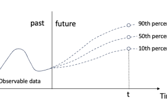
Today I would like to share a recent research work from the University of Connecticut that proposes a method to align time series data with large natural language processing (NLP) models on the latent space to improve the performance of time series forecasting. The key to this method is to use latent spatial hints (prompts) to enhance the accuracy of time series predictions. Paper title: S2IP-LLM: SemanticSpaceInformedPromptLearningwithLLMforTimeSeriesForecasting Download address: https://arxiv.org/pdf/2403.05798v1.pdf 1. Large problem background model
 Comparison summary of five deep learning models for time series forecasting
May 05, 2023 pm 05:16 PM
Comparison summary of five deep learning models for time series forecasting
May 05, 2023 pm 05:16 PM
The Makridakis M-Competitions series (known as M4 and M5 respectively) were held in 2018 and 2020 respectively (M6 was also held this year). For those who don’t know, the m-series can be thought of as a summary of the current state of the time series ecosystem, providing empirical and objective evidence for current theory and practice of forecasting. Results from the 2018 M4 showed that pure “ML” methods outperformed traditional statistical methods by a large margin that was unexpected at the time. In M5[1] two years later, the highest score was with only “ML” methods. And all the top 50 are basically ML based (mostly tree models). This game saw LightG
 Ten Python libraries recommended for time series analysis in 2022
Apr 13, 2023 am 08:22 AM
Ten Python libraries recommended for time series analysis in 2022
Apr 13, 2023 am 08:22 AM
A time series is a sequence of data points, usually consisting of consecutive measurements taken over a period of time. Time series analysis is the process of modeling and analyzing time series data using statistical techniques in order to extract meaningful information from it and make predictions. Time series analysis is a powerful tool that can be used to extract valuable information from data and make predictions about future events. It can be used to identify trends, seasonal patterns, and other relationships between variables. Time series analysis can also be used to predict future events such as sales, demand, or price changes. If you are working with time series data in Python, there are many different libraries to choose from. So in this article, we will sort out the most popular libraries for working with time series in Python. S
 Detailed explanation of ARMA model in Python
Jun 10, 2023 pm 03:26 PM
Detailed explanation of ARMA model in Python
Jun 10, 2023 pm 03:26 PM
Detailed explanation of the ARMA model in Python The ARMA model is an important type of time series model in statistics, which can be used for prediction and analysis of time series data. Python provides a wealth of libraries and toolboxes that can easily use the ARMA model for time series modeling. This article will introduce the ARMA model in Python in detail. 1. What is the ARMA model? The ARMA model is a time series model composed of an autoregressive model (AR model) and a moving average model (MA model). Among them, the AR model
 Graph-aware contrastive learning improves multivariate time series classification effects
Feb 04, 2024 pm 02:54 PM
Graph-aware contrastive learning improves multivariate time series classification effects
Feb 04, 2024 pm 02:54 PM
This paper in AAAI2024 was jointly published by the Singapore Agency for Science, Technology and Research (A*STAR) and Nanyang Technological University, Singapore. It proposed a method of using graph-aware contrastive learning to improve multivariate time series classification. Experimental results show that this method has achieved remarkable results in improving the performance of time series classification. Picture paper title: Graph-AwareContrastingforMultivariateTime-SeriesClassification Download address: https://arxiv.org/pdf/2309.05202.pdf Open source code: https://github.com/Frank-Wa
