
This article has compiled 10 of the most commonly used excel formulas for professionals. I hope it can help you solve your problems. Come and take a look!

Formula 1: Conditional Counting
Conditional counting is very common in Excel applications. For example, the number of women in the statistical list of personnel is the condition. Typical representation of counting.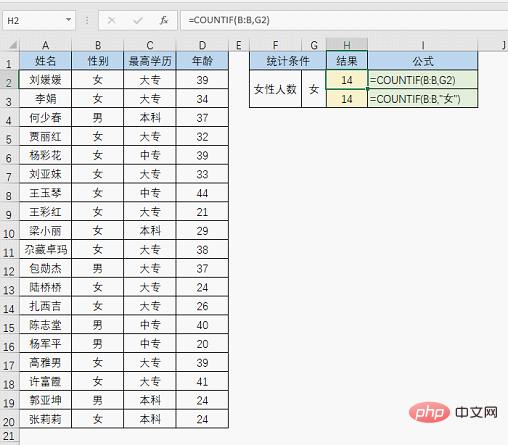
=COUNTIF (statistical area, condition). In this example, the first formula =COUNTIF(B:B,G2), B:B is the statistical area, G2 is the condition, and the formula result indicates that there are 14 "female" data in column B.
= COUNTIF(B:B,"女")That's it.
Formula 2: Quickly mark duplicate data
In daily work, we often encounter the problem of marking duplicate values, for example, in a document In the sales detail table, mark the duplicate salesperson names.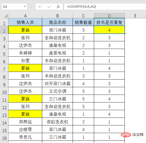
=COUNTIF(A:A,A2) to calculate the number of times each name appears. When the result is greater than 1, it means that the name is repeated. , and then use the IF function to get the final result.
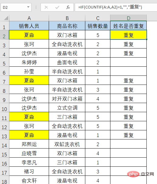
=IF(COUNTIF(A:A,A2)=1,"","Repeat"), the result is as shown in the figure.
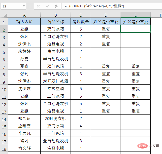
=IF(COUNTIF($A$1:A2,A2)=1,"","Repeat "), the result is as shown in the figure.
Formula 3: Multi-condition counting
If you want to count multiple conditions, you must Use the COUNTIFS function, for example, you need to count the number of men with a bachelor's degree in secondary school.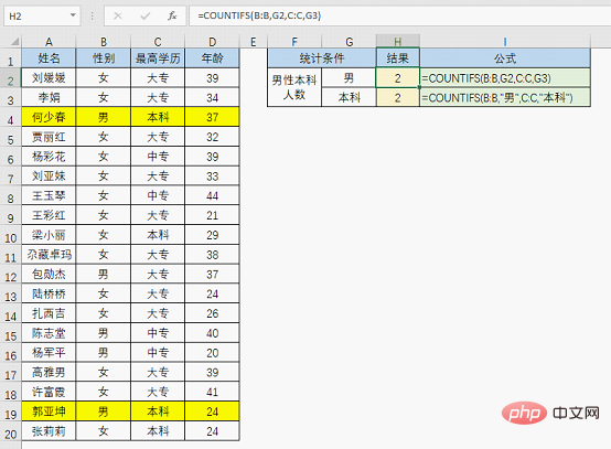
Formula 4: Conditional summation
In addition to conditional counting, conditional summation is also widely used, such as statistics in sales details Total TV sales.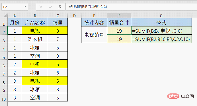
=SUMIF(B:B,B2,C:C).
Formula 5: Multi-condition summation
If there is a conditional summation, there will be a multi-condition summation, for example, based on salesperson and product When summing two conditions, the multi-condition summation function SUMIFS is used.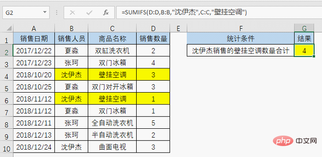
= SUMIFS(D:D,B:B,"Shen Yijie",C:C,"Wall-mounted air conditioner")
It should be reminded that the location of the summation area of SUMIFS is different from that of SUMIF. The summation area of SUMIFS is in the first parameter, while the summation area of SUMIF is in the third parameter. Don't get confused!
Formula 6: Calculate the date of birth based on the ID number
To get the date of birth from the ID number, this problem is very difficult for people who work Friends who are in administrative positions must be familiar with it, and the formula is relatively simple:
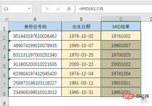
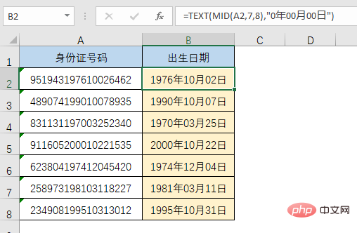
=TEXT(MID(A2,7,8),"0-00-00") to get the required results, as shown in the figure Shown:
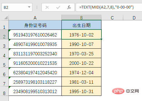
To understand the principle of this formula, you must first know some rules in ID numbers. The ID cards currently used are basically 18 digits. The eight digits starting with the seven digits represent the date of birth.
This formula involves two functions. First, let’s look at the MID function. The MID function has three parameters. The format is: =MID (where to extract, from which word to start, how many words to pick) .
MID(A2,7,8) means to intercept eight digits starting from the seventh number of cell A2. The effect is as shown in the figure:
After the birth date is extracted, it is not the effect we need. At this time, the function magician TEXT comes into play. The TEXT function has only two parameters, the format is =TEXT (the content to be processed, "in what format to display"), in this example The content to be processed is the MID function part. The display format is "0-00-00". Of course, it is no problem if you use the format of "0年00月00日". The formula is changed to =TEXT(MID(A2 ,7,8),"0年00月00日") will do:
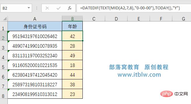
##Formula 7: Calculate age based on ID number
With the date of birth, of course you will think of calculating age. The formula is: =DATEDIF(B2,TODAY(),"Y")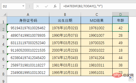
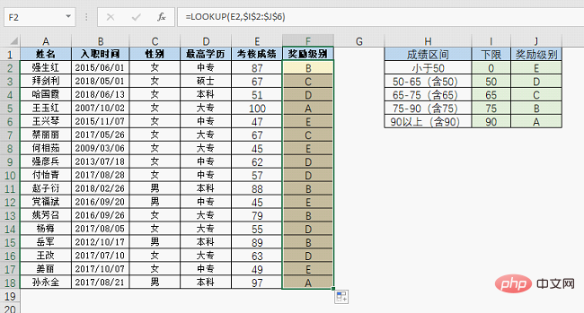
Formula 8: Different results are obtained according to the interval
This type of problem is often seen in performance appraisals. For example, when a company conducts performance appraisals for employees, it needs to determine the reward level based on the appraisal results. The grading rules are: E for scores below 50, D for 50-65 (inclusive), and D for 65-75 (inclusive). ) is C, 75-90 (inclusive) is B, and above 90 is A. You can use the formula =LOOKUP(E2,{0;50;65;75;90},{"E";"D";"C";"B";"A"}) to get each The reward level of each employee, the result is as shown in the figure: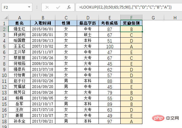
Formula 9: Single condition matching data
If you want to dominate the workplace, what can you do if you don’t know how to match? ? How can I do single condition matching without VLOOKUP? The basic structure of the VLOOKUP function is =VLOOKUP (what to look for, where to look for it, which column to look for, how to look for it). For example, to find the highest educational level by name, you can use the formula =VLOOKUP(G2,B:E,4 ,0) Get the desired result, as shown in the figure: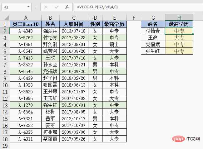
②The column number refers to the column in the search range rather than the column in the table. For example, if you want to find the highest educational level, you should find the 4th column in the search range, not the column number 5 in the table.
Formula 10: Multi-condition matching data
If you learn to match data with multiple conditions, you will be truly invincible!
Give an example of matching sales quantity by name and product name, as shown in the figure:

The formula is =LOOKUP( 1,0/(($A$2:$A$10=E2)*($B$2:$B$10=F2)),$C$2:$C$10)
Use the LOOKUP function The routine for multi-condition matching is: =LOOKUP(1,0/((search range 1=lookup value 1)*(search range 2=lookup value 2)*……*(search range n=lookup value n)), Result range), it should be noted that there is a multiplication relationship between multiple search conditions, and they need to be placed in the same set of brackets as the denominator of 0/.
Okay, the ten most commonly used formulas are shared here. If you use them well, you can really dominate the workplace!
Related learning recommendations: excel tutorial
The above is the detailed content of Practical Excel skills sharing: 10 most commonly used formulas among professionals. For more information, please follow other related articles on the PHP Chinese website!
 Compare the similarities and differences between two columns of data in excel
 excel duplicate item filter color
 How to copy an Excel table to make it the same size as the original
 Excel table slash divided into two
 Excel diagonal header is divided into two
 Absolute reference input method
 java export excel
 Excel input value is illegal


![[Web front-end] Node.js quick start](https://img.php.cn/upload/course/000/000/067/662b5d34ba7c0227.png)


