CMU Zhang Kun: Latest progress in causal representation technology

1. Why care about causality
First of all, let’s introduce what is causality:
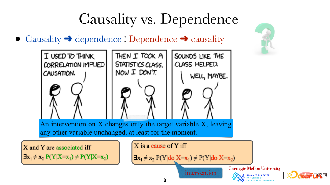
When we say There is a relationship between variables/events, which means that they are not independent, so there must be some relationship between them. However, the meaning of X being the "cause" of Y is that if a specific method is used to change Different. It should be noted that the intervention here is not random, but a very precise direct control of the target variable (directly changing "it rains"). This change will not directly affect other variables in the system. At the same time, in this way, that is, direct human intervention, we can also determine whether one variable is the direct cause of another variable.
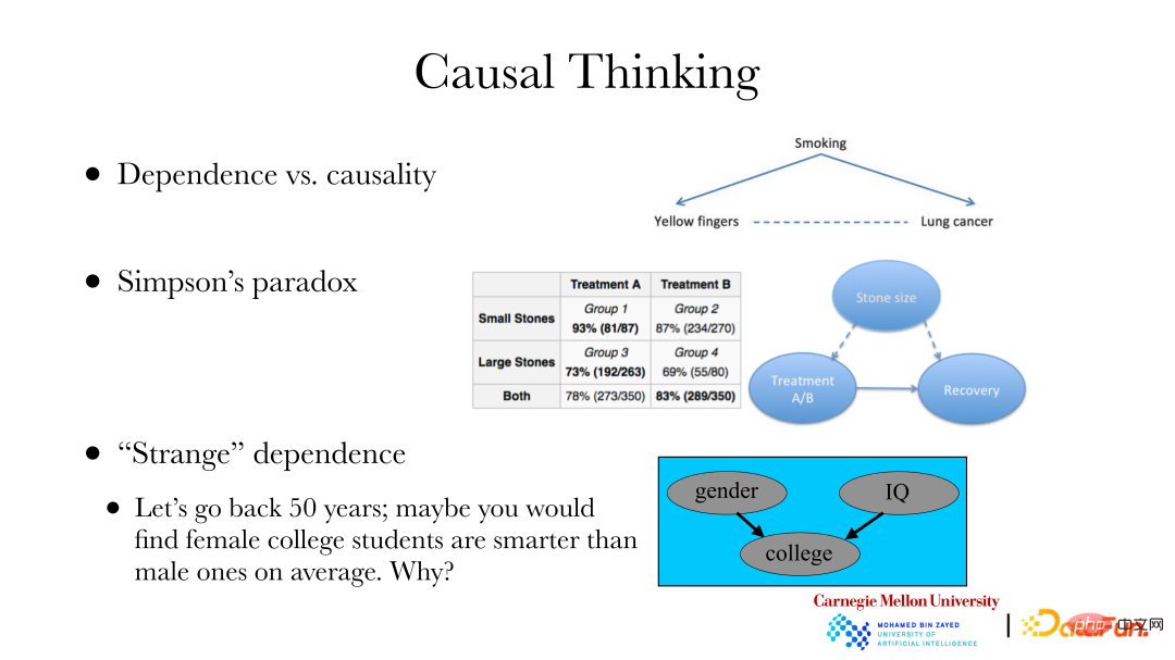
The following is an example of the need to analyze the causal relationship:
① A classic case is: lung disease and nail color exist through smoking. The relationship is that because cigarettes do not have filters, regular smoking will turn your fingernails yellow, and smoking may also cause lung disease. If you want to change the incidence of lung disease in a certain area, it cannot be improved by bleaching your nails. You need to find the cause of the lung disease, rather than changing the dependence of the lung disease. To achieve the goal of changing the incidence of lung disease, a causal analysis is needed.
② The second case is: Simpson's Paradox. The right side of the picture above is a real data set. The data set shows two sets of kidney stone data, one group has smaller stones and the other has larger stones; in addition, there are two treatment methods A and B. It can be found in the table that regardless of the small stone group or the large stone group, the results obtained by treatment method A are better, with cure rates of 93% and 73% respectively, and the cure rates of treatment method B are 87% and 69% respectively. However, when two groups of stone patients with the same treatment method were mixed together, the overall effect of treatment plan B (83%) was better than that of treatment plan A (78%). Suppose you are a doctor who only cares about the cure rate, how to choose a treatment plan for new patients. The reason for this is that when making recommendations, we only care about the causal link between treatment and cure, and do not care about other dependencies. However, stone size is a common cause of both treatment and whether it is cured, which leads to quantitative changes in the dependence of treatment and cure. Therefore, when studying the relationship between treatment methods and cure, we should discuss the causal relationship between the former and the latter, rather than the dependence relationship.
③ The third case: 50 years ago, statistics showed that women in colleges and universities were on average smarter than men, but in reality there should not be a significant difference. There is a selection bias, because it is more difficult for women to enter college than men. That is, when schools recruit students, they will be affected by factors such as gender and test ability. When the "result" has occurred, there will be some relationship between gender and examination ability. The problem of selection bias also exists when using data collected from the Internet. There is often a relationship between whether a data point is collected and certain attributes. If you only analyze data placed on the Internet, you need to pay attention to these factors. When this is realized, data with selection bias can also be analyzed through causal relationships, and then the nature of the entire group itself can be restored or inferred.
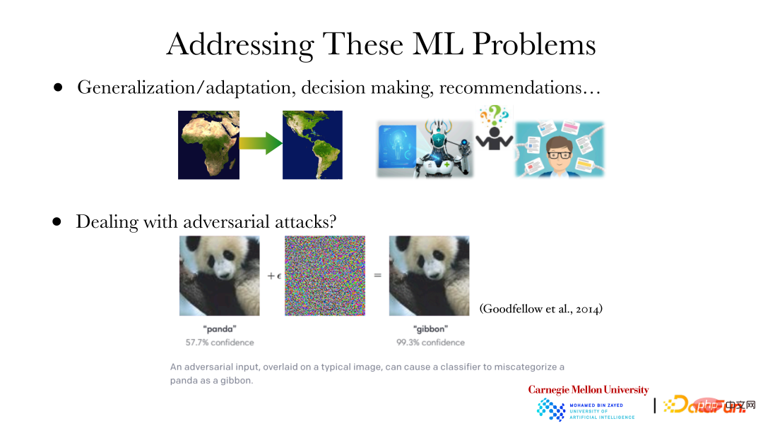
The above figure shows several machine learning/deep learning problems:
① We know that the most prediction is related to the distribution of data. In transfer learning, for example, if you want to transfer a model from Africa to the Americas and still make optimal predictions, this obviously requires adaptive adjustments of the model based on different data distributions. At this time, it is particularly important to analyze what changes have occurred in the distribution of data and how they have changed. Knowing what has changed in the data allows you to adjust the model accordingly. Another example, when building an AI model to diagnose a disease, you will not be satisfied with the diagnosis results proposed by the machine. You will further want to know why the machine came to this conclusion, such as which mutation caused the disease. Additionally, how to treat a disease raises many "why" questions. Similarly, when a recommendation system makes a recommendation, it will want to know why it recommends this item/strategy, for example, the company just wants to increase revenue, or the item/strategy is suitable for the user, or the item/strategy is beneficial to the future. These "why" questions are all cause and effect questions.
② In the field of deep learning, there is the concept of adversarial attacks. As shown in the figure, if you add some specific noise to the giant panda picture on the left, or change specific pixels, etc., the machine will judge the picture as other types of animals instead of giant pandas, and its confidence level is still very high. However, to humans, these two pictures are obviously giant pandas. This is because the high-level features currently learned by machines from images do not match the high-level features learned by humans. If the high-level features used by machines do not match those of humans, adversarial attacks may occur. When the input is changed, the judgment of humans or machines will change, and there will be problems with the final judgment result. Only by allowing the machine to learn high-level features that are consistent with humans, that is, the machine can learn and use features in the same way as humans, can we avoid adversarial attacks.
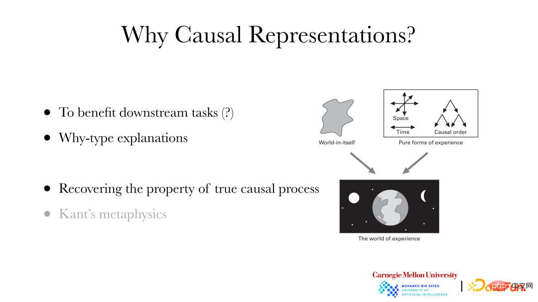
Why do we need to carry out causal representation?
① Benefit downstream tasks: For example, it can help downstream classification and other tasks to do better.
② Can explain “why” questions.
③ Recover the real causal characteristics behind the data: Kant’s metaphysics in philosophy believes that the world experienced by humans is the empirical world. Although it is based on the world-in-itself behind it, we cannot directly perceive the world ontology. Some properties, such as time, space, causal order, etc., have been automatically added to the experiential world by the sensory system. Therefore, if you want a machine to learn features consistent with humans, you need the machine to have the ability to learn features such as causal order/relationship, time, and space.
2. Causal representation learning: independent and identically distributed situation
1. Basic concepts of causal representation learning
How to learn causal relationships in the independent and identically distributed situation? First, two questions need to be answered: First, what properties in the data are related to causality, and what clues ("footprint") are there in the data. The second is whether the causal relationship can be recovered under the conditions of obtaining the data, that is, the issue of the identifiability of the causal system.
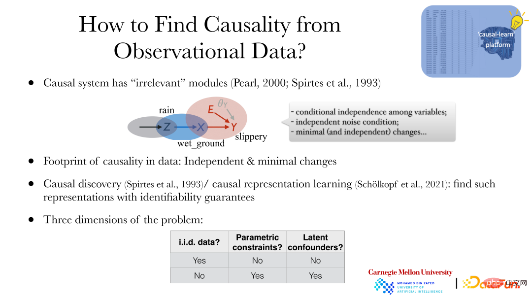
The most essential property of a causal system is "modularity": Although the variables in the system have certain relationships, the system can be divided into causal relationships. Multiple subsystems (one cause produces one dependent variable). For example, "It's raining", "The ground is wet", and "The ground is slippery" are interdependent and can be divided into three subsystems through causal relationships: "Some reasons cause it to rain", "It rains to cause the ground to be wet" , "The wet ground causes the ground to be slippery." Although there are dependencies between variables, these three processes (processes, subsystems) are not connected, there is no parameter sharing, and changes in one system will not cause changes in the other system. For example, by spraying certain substances to change the effect of "wet ground causing slippery ground", this will not affect whether it rains or not, nor will it change the effect of rain on the ground being wet. This property is called "modularity", which means that the system is divided into different sub-modules from a causal perspective, and there is no connection between the sub-modules.
Starting from modularity, we can get three properties of causal systems:
① Conditional independence between variables.
② Independent noise condition.
③ Minimal (and independent) changes.
Regarding the identifiability of causal systems, generally speaking, machine learning itself does not pay much attention to the issue of identifiability. For example, the prediction model needs to judge whether the prediction result is accurate or optimal, but there is no "truth" for it. judge. However, causal analysis/causal representation learning is to restore the "truth" of the data, that is, it pays more attention to whether the causal nature behind the data can be identified.
Two basic concepts are introduced below:
① Causal discovery: Exploring the underlying causal structure/model through data.
② Causal representation learning: Find the underlying high-level hidden variables and relationships between variables from directly observed data.
2. Division of causal representation learning
Causal representation learning methods are generally divided from the following three perspectives:
① Data properties: whether they are independent and identically distributed ("i.i.d. data" ). The non-independent and identically distributed data includes non-independent but identically distributed data, such as identically distributed data with time dependence (such as time series data), or independent but differently distributed data, such as data distribution changes (or these two combination of those).
② Parameter constraints ("parameter constraints"): Whether there are other additional properties on the influence of causality, such as parameter models.
③ Potential confounding factors (“latent confounders”): Whether to allow the existence of unobserved common factors or confounding factors in the system.
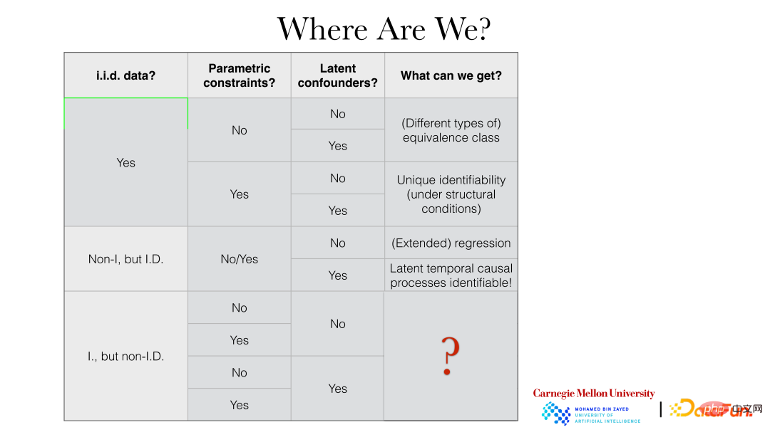
The following figure shows in detail the specific results that can be obtained under different settings:
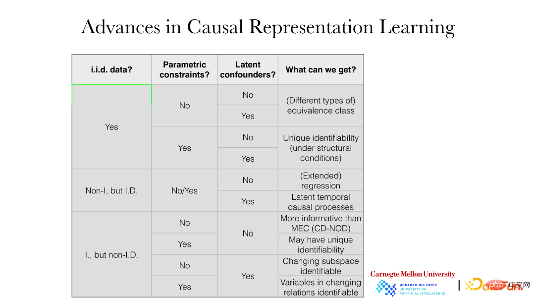
For example, in the case of independent and identical distribution, if there is no parameter model Constraints, regardless of whether there are potential confounding factors, can generally obtain equivalence classes ("equivalence classes"). If there are parametric model constraints, the truth behind them can generally be directly restored.
3. Independent and identically distributed causal representation learning
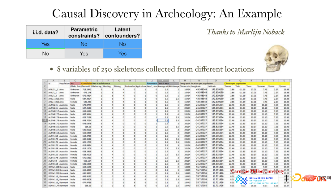
The above figure shows an example without parameter model constraints in the independent and identically distributed situation. The data shows a total of 8 measured variables for 250 skulls, including gender, location, weather, and skull size and shape. Archaeologists want to know what causes the different appearances of people in different areas. If we know this causal relationship, we may be able to predict people's appearance through changes in the environment and other factors. Obviously, human intervention cannot be carried out under such conditions. Even if intervention is added, it will take a long time to observe the results. Therefore, the causal relationship can only be found from the existing observation data.
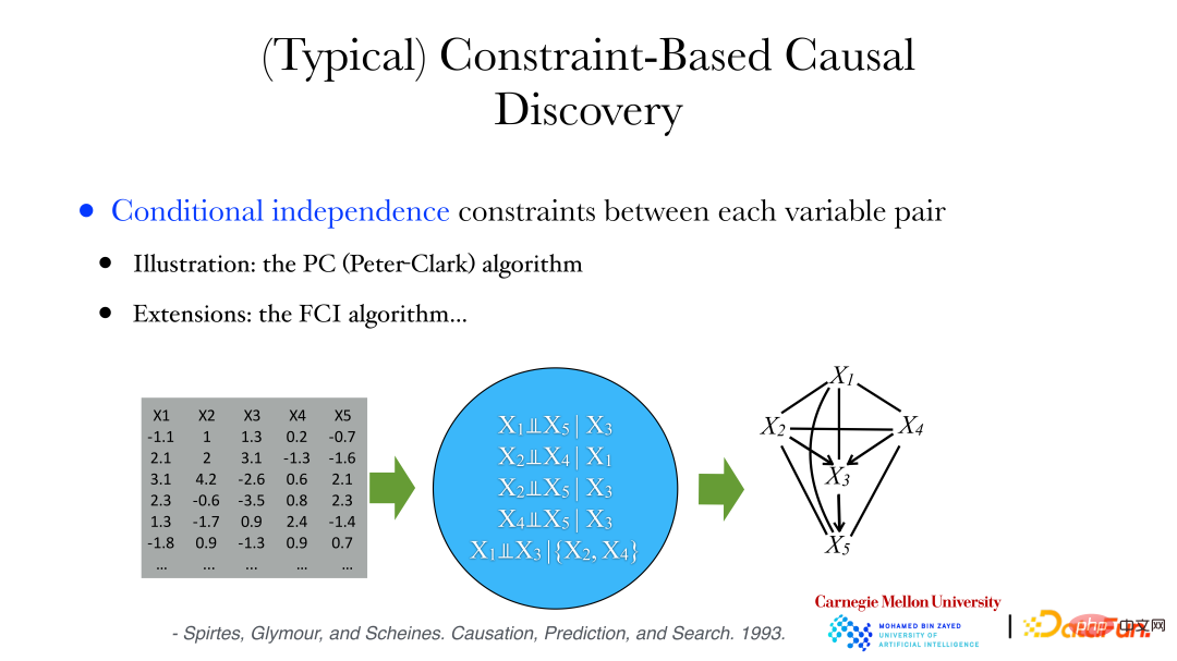
As shown in the figure above, the relationship between variables is very complex, it may be linear or nonlinear, and the variable dimensions may also be inconsistent. If gender is 1 dimension, skull traits might be 255 dimensions. At this time, the property of conditional independence can be used to construct causal relationships.
Methods include the following two types:
① PC (Peter-Clark) algorithm: The algorithm assumes that no common factors are observed in the system.
② FCI algorithm: used when there are hidden variables.
The PC algorithm will be used to analyze archaeological data below: a series of conditionally independent properties can be derived from the data, such as variables X1 and X5 being conditionally independent when X3 is given, etc. At the same time, we can prove that if two variables are conditionally independent, then there is no edge between them. Then, we can start from the complete graph. If the variables are conditionally independent, then remove the connected edges to get an undirected graph. Then judge the direction of the edges in the graph to find the directed acyclic graph. (DAG, Directed Acyclic Graph) or a collection of directed acyclic graphs to satisfy the conditional independence constraints between variables in the data.
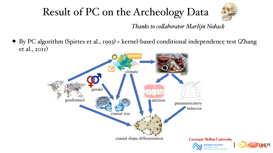
The above figure shows the results of analyzing archaeological data using the PC algorithm and the kernel conditional independence test method: geographical location affects weather, weather affects skull size, and gender also Can affect skull size etc. The causal relationship behind it was obtained through data analysis.
Among the two problems just mentioned, one is to find the direction of each edge of the variable DAG, which requires additional assumptions. If you make some assumptions about how cause affects effect, you will find that cause and effect are asymmetrical, so you can find out the direction of cause and effect. The data background in the figure below is still independent and identically distributed data, and additional parameter restrictions have been added, and confounding factors are still not allowed in the system. At this time, the following three types of models can be used to study the causal direction:
① Linear non-Gaussian model;
② Post-nonlinear causal model (PNL, Post -nonlinear causal model);
③ Additive noise model (ANM, Additive noise model).
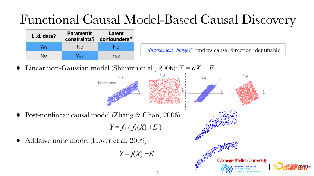
In the linear non-Gaussian model, it is assumed that X leads to Y, that is, X is the dependent variable and Y is the effect variable. It can be seen from the figure that when using X to explain Y for linear regression, the residuals and X are independent; but conversely, when using Y to explain Obviously they are not independent (in the case of linear Gaussian, uncorrelatedness between variables means independence. But at this moment the model is linear non-Gaussian, that is, uncorrelated does not mean they are independent). It can be found that there is an asymmetry between the dependent variable and the effect variable. The same applies to post-nonlinear causal models and additive noise models.
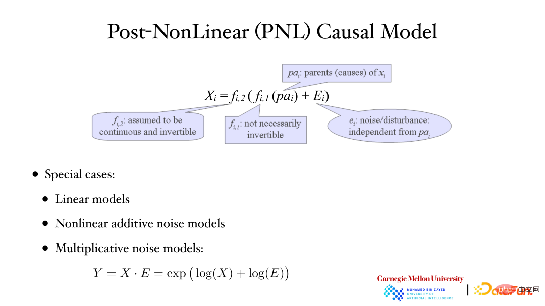
The above figure shows the post-nonlinear causal model: the second nonlinear function (f2) outside is generally used to describe the non-linear factors introduced in the measurement process in the system. Linear changes, there are often non-linear changes when observing/measuring data. For example, in the biological field, there will be additional non-linear changes when using instruments to measure gene expression data. Linear models, nonlinear additive noise models, and multiplicative noise models are all special cases of PNL models.
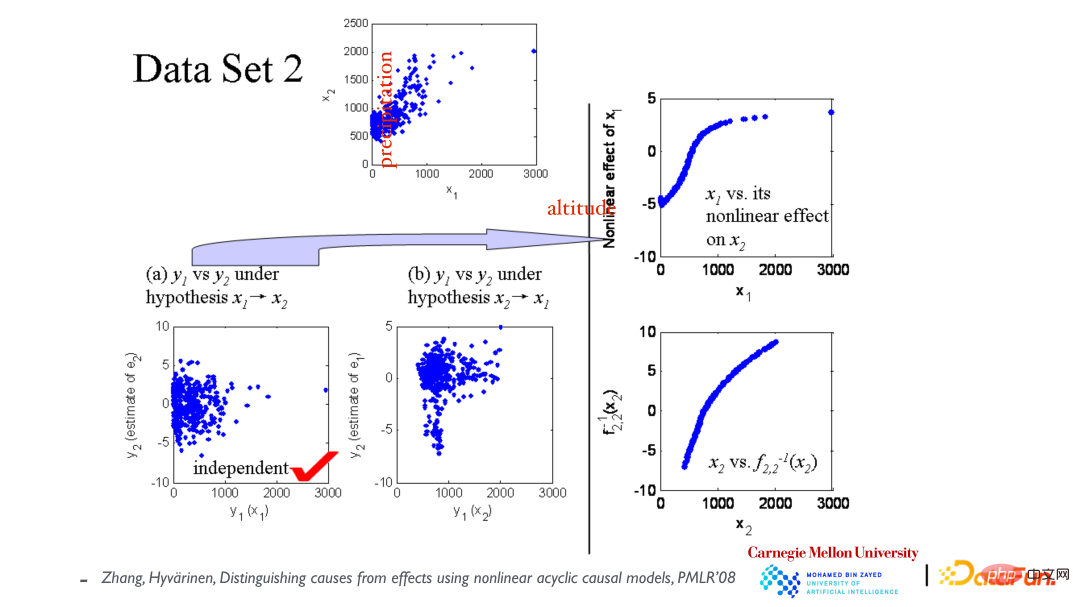
The top scatter plot shows the relationship between the variables x1 (elevation) and x2 (annual rainfall). First assume that x1 causes x2, and then build a model to fit the data. As shown in the lower left corner, the residuals and x1 are independent; then assume that x2 causes x1, and fit the model again. We find that the residuals and x2 are not Independent (see middle picture). From this, it is concluded that the causal direction is caused by x1 leading to x2.
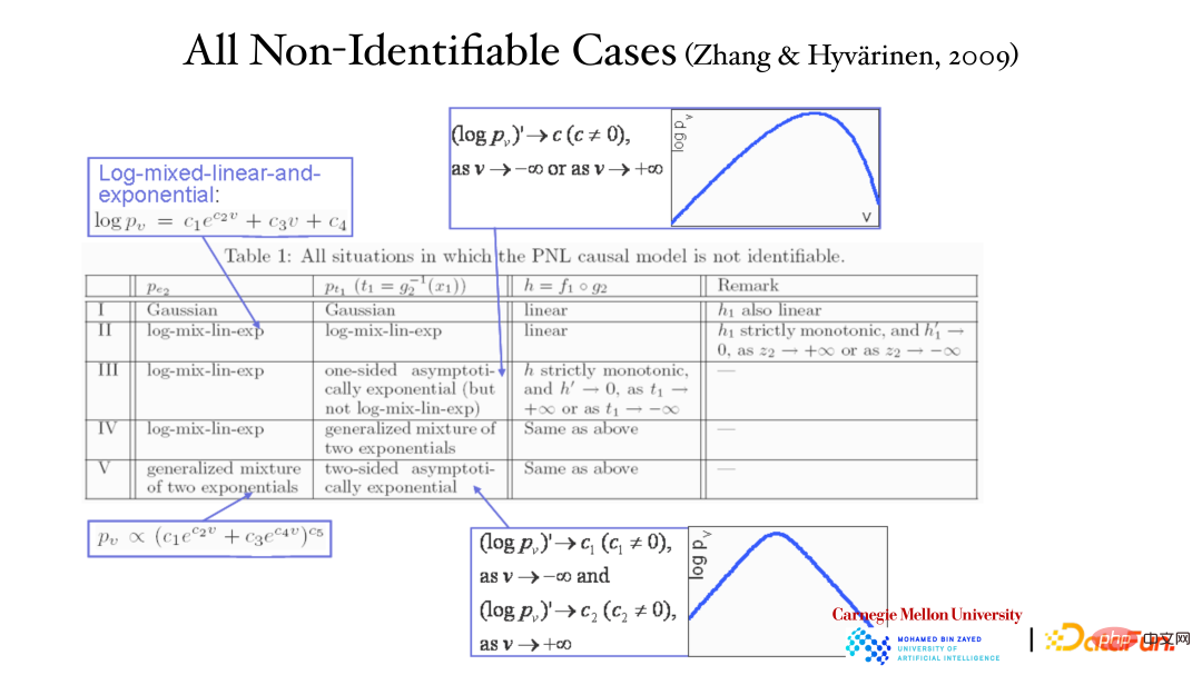
It is true that the asymmetry of the causal variables can be found from the previous example, but can this result be guaranteed theoretically? And it is the only correct result. The opposite direction (effect to cause) cannot explain the data? The proof is as shown in the table above. In five cases, the data can be explained in both directions (cause to effect, effect to cause). These five are very special cases. The first is the linear Gaussian model, where the relationship is linear and the distribution is Gaussian, where the causal asymmetry disappears. The other four are special models.
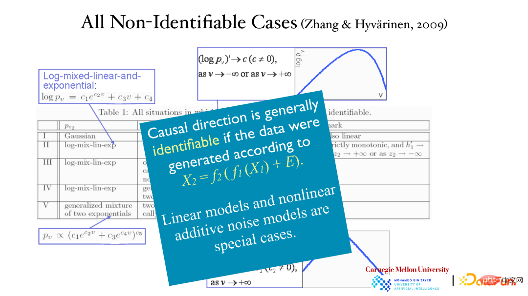
Even if the data is analyzed using a post-nonlinear model, cause and effect can be distinguished. Independent residuals can be found in the correct direction, but not in the opposite direction. Arrived. Since the linear model and the nonlinear additive noise model are both special cases of the post-nonlinear model, both models are also applicable in this case and can find the causal direction.
Given two variables, their causal directions can be found through the above method. But in more cases, the following problems need to be solved: For example, in the field of psychology, answers to some questions (xi) are collected through questionnaires. There is a dependence between these answers, and it is not considered that there is a relationship between these answers. direct causal relationship.
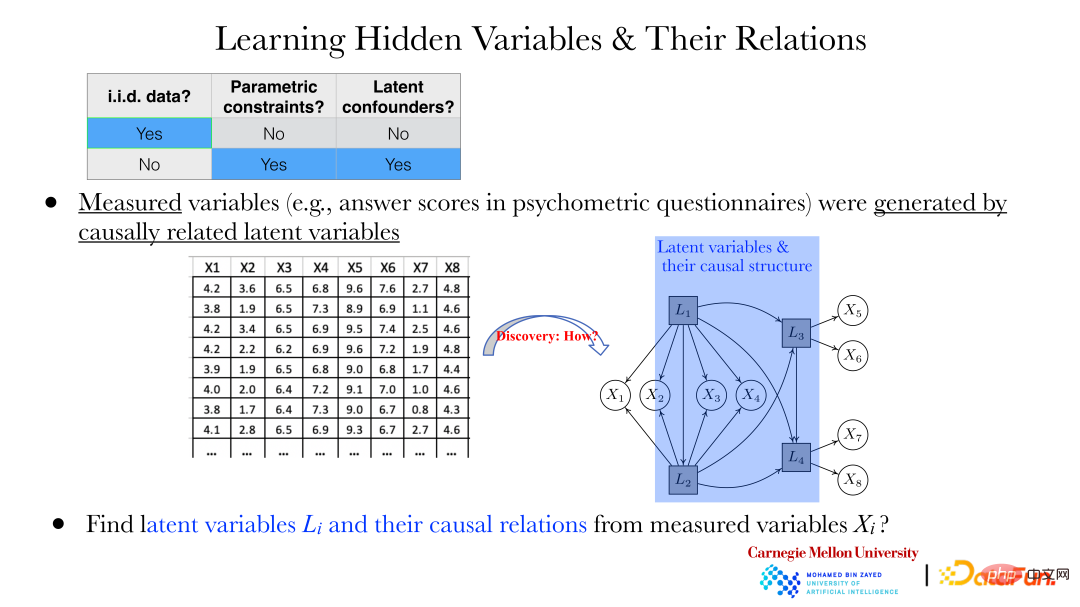
But as shown in the figure above, these xi are generated together with the hidden variables Li behind them. How to reveal the hidden variables Li and the relationship between hidden variables through the observed xi is particularly important.
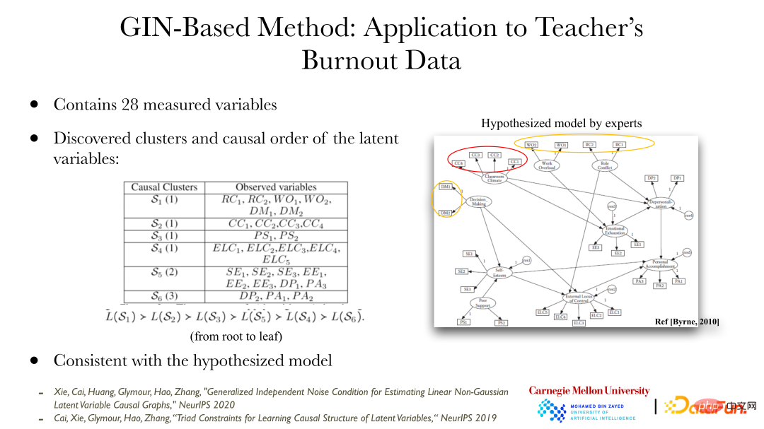
In recent years, there have been some methods that can help us find these dependent variables and their relationships. The figure above shows an application example of the Generalized Independent Noise (GIN) method, which can solve a series of problems. The data content is teachers’ professional burnout, which contains 28 variables. The figure on the right shows the possible latent variables proposed by experts that lead to these burnout conditions (observed variables), and the relationship between the latent variables. The results obtained by analyzing the observed data through the GIN method are consistent with the results given by the experts. Experts conduct analysis through qualitative background knowledge, and the quantitative analysis method of data analysis provides verification and support for expert results.
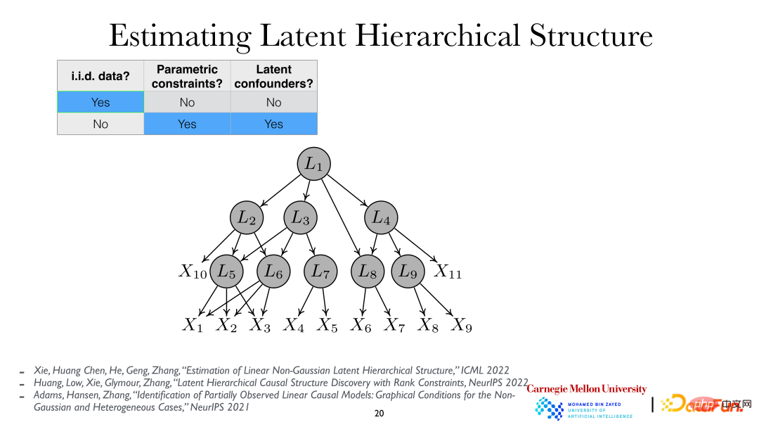
#For further in-depth analysis, we can assume that the latent variables are hierarchical, that is, the latent variable hierarchical structure (Latent Hierarchical Structure). By analyzing the observed variables xi, the hidden variables Li and their relationships behind them can be revealed.
3. Causal representation learning from time series
Now that we understand the causal representation method under independent and identically distributed situations, we will introduce how to use independent and identically distributed methods under nonlinear conditions. How to find the hidden variables and causal relationships behind it. Generally speaking, in the case of independent and identical distribution, relatively strong conditions (including parametric model assumptions, linear models, sparse graphs, etc.) are required to find the causal relationship. In other cases, causation can be found more easily.
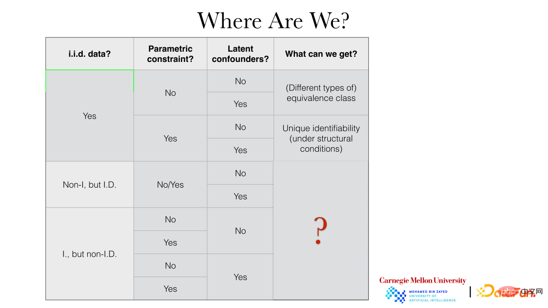
The following will introduce how to find causal representations from time series, that is, how to perform causal analysis when the data are not independent but identically distributed:
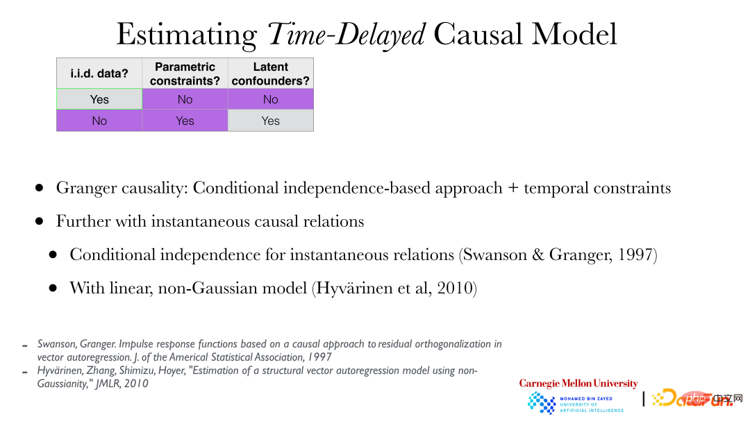
If causality occurs in the observed time series, this is a classic problem of finding causality from time series data, that is, Granger causality. Granger causality is consistent with the previously mentioned causality based on conditional independence, but with the addition of time constraints (if it cannot occur earlier than the cause), and furthermore, instantaneous causal relations can be introduced. .
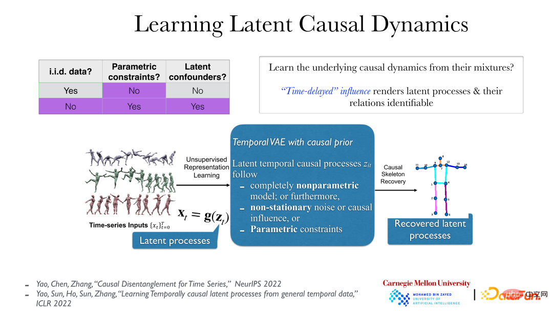
The above picture shows a more practical method. In video data, the truly meaningful latent process behind the data is that the data we observe, as their reflection, are generated by their transformation by a reversible smooth nonlinear function. The real implicit causal process generally has a causal connection in time, such as "push and then fall". This causal effect is generally time-delayed. Under these conditions, even under very weak assumptions (even if the underlying latent process is non-parametric and the g function (from the latent process to the observed time series) is also non-parametric), the underlying latent process can be completely understood All revealed.
This is because after returning to the real implicit process, there is no instantaneous causality and dependence, and the relationship between objects will be clearer. However, if you use the wrong analysis method to look at the observation data, such as directly observing the pixels of the video data, you will find that there is an instantaneous dependency between them.
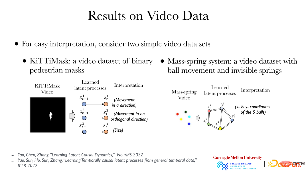
The above figure shows two simple cases: the left side shows the KiTTiMask video data. Analyzing the video data, we get three implicit processes: moving in one direction; moving in the vertical direction; and changing the mask size. The right side shows 5 small balls of different colors. Some balls are connected by springs (invisible). Through analysis, 10 hidden variables (x, y coordinates of the 5 small balls) can be obtained, and then the cause and effect between them can be found. relationship (there are springs between some balls). Based on video data, we can directly use a completely unsupervised method and introduce the principle of cause and effect to find the relationship between the objects behind it.
4. Causal representation learning under multiple distributions
Finally, let’s introduce the causal analysis when the data distribution changes:
When When recording variables/processes over time, it is often found that the data distribution changes over time. This is due to changes in the value of the underlying unobserved/measured variable, thereby changing the data distribution of the observed variable in response. Similarly, if you measure data under different conditions, you will find that the distribution of data measured under different conditions/locations may also be different.
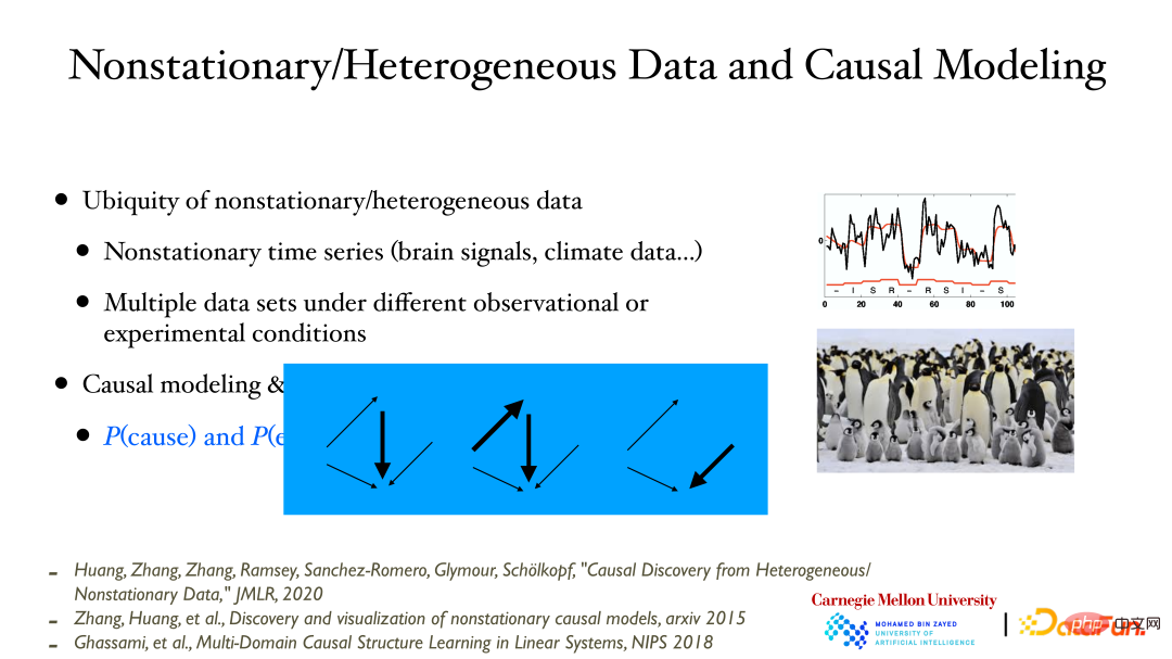
The point to be emphasized here is that there is a very close connection between causal modeling and changes in data distribution. When a causal model is given, based on the modular nature, these sub-modules can change independently. If this change can be observed from the data, the correctness of the causal model can be verified. The change of the causal model mentioned here means that the causal influence can become stronger/weaker or even disappear.
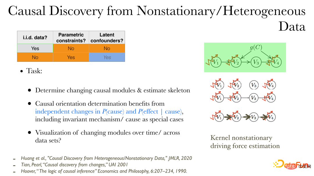
In nonstationary data/heterogeneous data, causal relationships can be discovered more directly. After the observed variables are given:
① First, you can observe which variables will change in their causal production process;
② Determine the undirected edges (skeleton) of the causal influence;
③ Find out the direction of causation: When the data distribution changes, additional properties can be used: changes in the cause and changes in the effect according to the cause are independent and unconnected. Because the changes between different modules are independent;
④ Use low-dimensional visualization methods to describe the process of causal changes.
The following figure shows some results of analyzing stock daily return data (instantaneous data, no time lag) in the New York Stock Exchange:
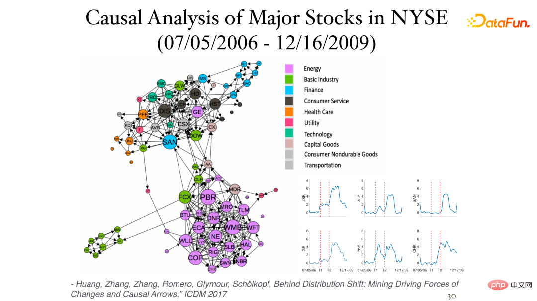
The influence of the asymmetry between them can be found through non-stationarity. Different sectors are often in a cluster and are closely related. The image in the lower right corner shows the causal process of stock changes over time, with the two vertical axes representing the financial crises of 2007 and 2008 respectively.
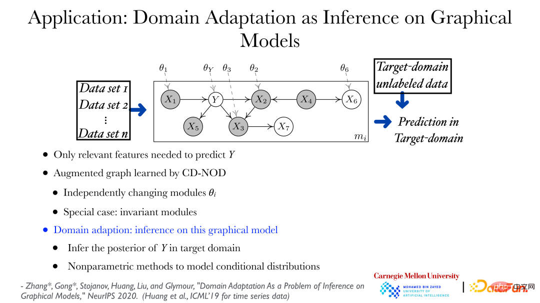
Through the causal analysis method under multi-distribution conditions, the changing patterns of data can be found from different data sets, and direct application can be used to perform transfer learning and domain adaptation. ). As shown in the figure above, you can find out the changing rules of data from different data sets, and use an augmented graph to show how the distribution of data can change. In the figure, theta_Y represents, Y is giving it The distribution under the parent node can change according to its domain. Based on the graph describing the changes in the data distribution, predicting Y in a new field or target field is a very standard problem. That is, how to find the posterior probability of Y given the feature value is an inference problem. .
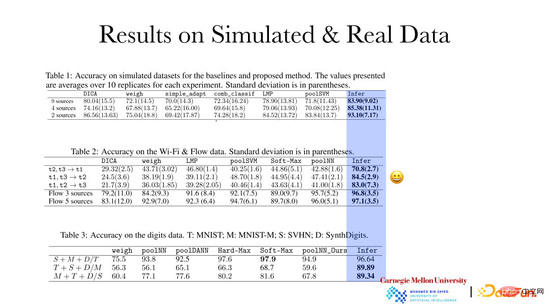
The above figure shows that the accuracy of the reasoning effect of the causal representation method on simulated data and real data has been significantly improved. Based on the qualitative change rules and the magnitude of variability in different fields, adaptive adjustments will be made when new fields emerge. This kind of prediction effect will be better.
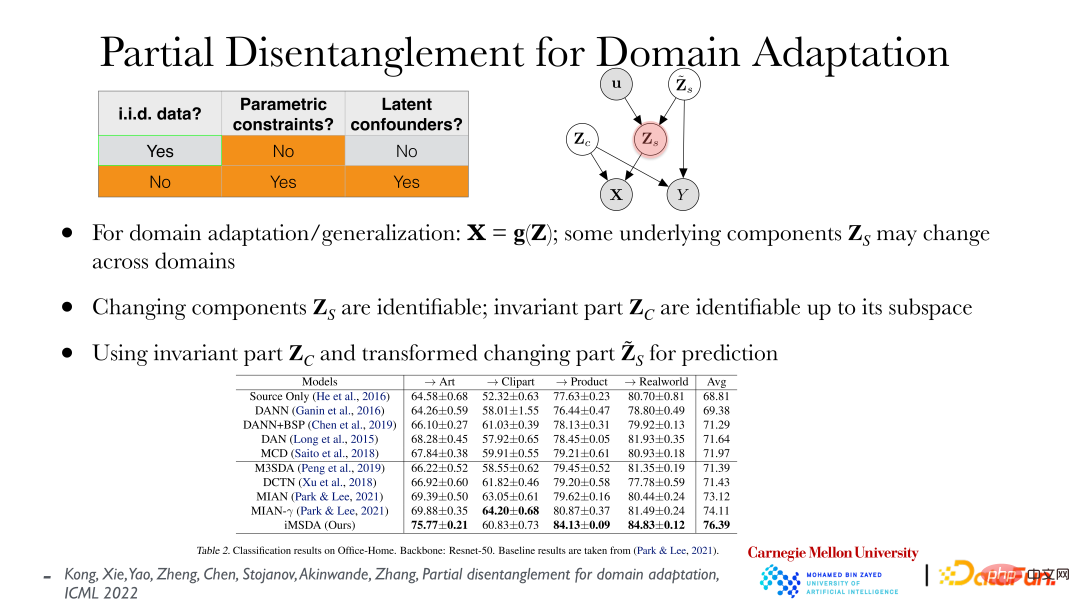
The above figure shows recent work related to Partial Disentanglement for Domain Adaption. Given the feature and target, assume that everything is non-parametric, and some factors do not change with the domain, that is, the distribution is stable, but some factors may change. Hope to find these very few factors that change the distribution. Based on the found factors, different fields can be aligned together, and then the corresponding relationships between different fields can be found, so that domain adaptation/transfer learning will be a matter of course. It can be proved that the independent factors behind the changes in the distribution can be directly recovered from the observation data, and the unchanged factors can restore their subspace. As shown in the table, the above methods can achieve good results in domain adaptation. At the same time, this method also conforms to the principle of minimal change, that is, it is hoped to use the least changed factor to explain how the factors of data in different fields have changed, so as to correspond them.
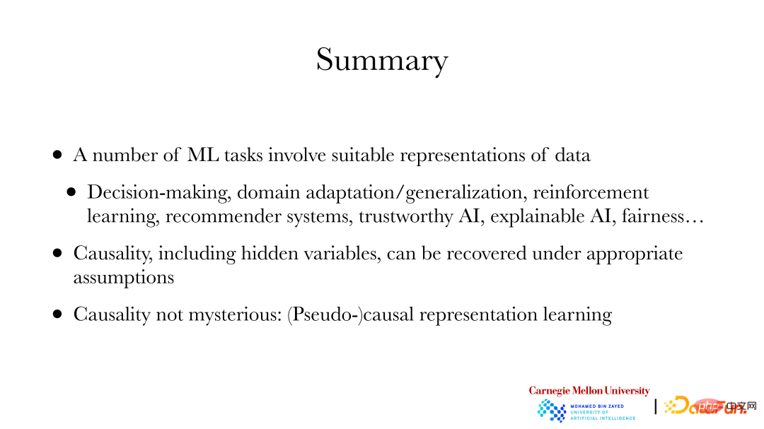
To summarize, this sharing mainly includes the following content:
① A series of machine learning problems require a suitable representation behind the data. For example, when making a decision, you want to know the impact of the decision, so that you can make the optimal decision; in domain adaptation/generalization, you want to know how the distribution of the data has changed, so as to make the optimal prediction; in reinforcement learning, the agent The interaction with the environment and the reward brought by the interaction itself is a causal problem; the recommendation system is also a causal problem, because the user is changed; trustworthy AI, explainable AI, and fairness are all related to causal representation.
② Causality, including hidden variables, can be completely recovered from the data under certain conditions. You can really understand the nature of the process behind it through the data and then use it.
③ The relationship between cause and effect is not mysterious. As long as there is data and the hypothesis is appropriate, the causality behind it can be found. The assumptions made here should preferably be testable.
In general, causal representation learning has great application prospects. At the same time, there are many methods that need to be developed urgently and require joint efforts by everyone.
The above is the detailed content of CMU Zhang Kun: Latest progress in causal representation technology. For more information, please follow other related articles on the PHP Chinese website!

Hot AI Tools

Undresser.AI Undress
AI-powered app for creating realistic nude photos

AI Clothes Remover
Online AI tool for removing clothes from photos.

Undress AI Tool
Undress images for free

Clothoff.io
AI clothes remover

AI Hentai Generator
Generate AI Hentai for free.

Hot Article

Hot Tools

Notepad++7.3.1
Easy-to-use and free code editor

SublimeText3 Chinese version
Chinese version, very easy to use

Zend Studio 13.0.1
Powerful PHP integrated development environment

Dreamweaver CS6
Visual web development tools

SublimeText3 Mac version
God-level code editing software (SublimeText3)

Hot Topics
 1378
1378
 52
52
 Methods and steps for using BERT for sentiment analysis in Python
Jan 22, 2024 pm 04:24 PM
BERT is a pre-trained deep learning language model proposed by Google in 2018. The full name is BidirectionalEncoderRepresentationsfromTransformers, which is based on the Transformer architecture and has the characteristics of bidirectional encoding. Compared with traditional one-way coding models, BERT can consider contextual information at the same time when processing text, so it performs well in natural language processing tasks. Its bidirectionality enables BERT to better understand the semantic relationships in sentences, thereby improving the expressive ability of the model. Through pre-training and fine-tuning methods, BERT can be used for various natural language processing tasks, such as sentiment analysis, naming
 Analysis of commonly used AI activation functions: deep learning practice of Sigmoid, Tanh, ReLU and Softmax
Dec 28, 2023 pm 11:35 PM
Activation functions play a crucial role in deep learning. They can introduce nonlinear characteristics into neural networks, allowing the network to better learn and simulate complex input-output relationships. The correct selection and use of activation functions has an important impact on the performance and training results of neural networks. This article will introduce four commonly used activation functions: Sigmoid, Tanh, ReLU and Softmax, starting from the introduction, usage scenarios, advantages, disadvantages and optimization solutions. Dimensions are discussed to provide you with a comprehensive understanding of activation functions. 1. Sigmoid function Introduction to SIgmoid function formula: The Sigmoid function is a commonly used nonlinear function that can map any real number to between 0 and 1. It is usually used to unify the
 Beyond ORB-SLAM3! SL-SLAM: Low light, severe jitter and weak texture scenes are all handled
May 30, 2024 am 09:35 AM
Written previously, today we discuss how deep learning technology can improve the performance of vision-based SLAM (simultaneous localization and mapping) in complex environments. By combining deep feature extraction and depth matching methods, here we introduce a versatile hybrid visual SLAM system designed to improve adaptation in challenging scenarios such as low-light conditions, dynamic lighting, weakly textured areas, and severe jitter. sex. Our system supports multiple modes, including extended monocular, stereo, monocular-inertial, and stereo-inertial configurations. In addition, it also analyzes how to combine visual SLAM with deep learning methods to inspire other research. Through extensive experiments on public datasets and self-sampled data, we demonstrate the superiority of SL-SLAM in terms of positioning accuracy and tracking robustness.
 Latent space embedding: explanation and demonstration
Jan 22, 2024 pm 05:30 PM
Latent Space Embedding (LatentSpaceEmbedding) is the process of mapping high-dimensional data to low-dimensional space. In the field of machine learning and deep learning, latent space embedding is usually a neural network model that maps high-dimensional input data into a set of low-dimensional vector representations. This set of vectors is often called "latent vectors" or "latent encodings". The purpose of latent space embedding is to capture important features in the data and represent them into a more concise and understandable form. Through latent space embedding, we can perform operations such as visualizing, classifying, and clustering data in low-dimensional space to better understand and utilize the data. Latent space embedding has wide applications in many fields, such as image generation, feature extraction, dimensionality reduction, etc. Latent space embedding is the main
 Understand in one article: the connections and differences between AI, machine learning and deep learning
Mar 02, 2024 am 11:19 AM
In today's wave of rapid technological changes, Artificial Intelligence (AI), Machine Learning (ML) and Deep Learning (DL) are like bright stars, leading the new wave of information technology. These three words frequently appear in various cutting-edge discussions and practical applications, but for many explorers who are new to this field, their specific meanings and their internal connections may still be shrouded in mystery. So let's take a look at this picture first. It can be seen that there is a close correlation and progressive relationship between deep learning, machine learning and artificial intelligence. Deep learning is a specific field of machine learning, and machine learning
 Super strong! Top 10 deep learning algorithms!
Mar 15, 2024 pm 03:46 PM
Almost 20 years have passed since the concept of deep learning was proposed in 2006. Deep learning, as a revolution in the field of artificial intelligence, has spawned many influential algorithms. So, what do you think are the top 10 algorithms for deep learning? The following are the top algorithms for deep learning in my opinion. They all occupy an important position in terms of innovation, application value and influence. 1. Deep neural network (DNN) background: Deep neural network (DNN), also called multi-layer perceptron, is the most common deep learning algorithm. When it was first invented, it was questioned due to the computing power bottleneck. Until recent years, computing power, The breakthrough came with the explosion of data. DNN is a neural network model that contains multiple hidden layers. In this model, each layer passes input to the next layer and
 From basics to practice, review the development history of Elasticsearch vector retrieval
Oct 23, 2023 pm 05:17 PM
1. Introduction Vector retrieval has become a core component of modern search and recommendation systems. It enables efficient query matching and recommendations by converting complex objects (such as text, images, or sounds) into numerical vectors and performing similarity searches in multidimensional spaces. From basics to practice, review the development history of Elasticsearch vector retrieval_elasticsearch As a popular open source search engine, Elasticsearch's development in vector retrieval has always attracted much attention. This article will review the development history of Elasticsearch vector retrieval, focusing on the characteristics and progress of each stage. Taking history as a guide, it is convenient for everyone to establish a full range of Elasticsearch vector retrieval.
 AlphaFold 3 is launched, comprehensively predicting the interactions and structures of proteins and all living molecules, with far greater accuracy than ever before
Jul 16, 2024 am 12:08 AM
Editor | Radish Skin Since the release of the powerful AlphaFold2 in 2021, scientists have been using protein structure prediction models to map various protein structures within cells, discover drugs, and draw a "cosmic map" of every known protein interaction. . Just now, Google DeepMind released the AlphaFold3 model, which can perform joint structure predictions for complexes including proteins, nucleic acids, small molecules, ions and modified residues. The accuracy of AlphaFold3 has been significantly improved compared to many dedicated tools in the past (protein-ligand interaction, protein-nucleic acid interaction, antibody-antigen prediction). This shows that within a single unified deep learning framework, it is possible to achieve


