
 Topics
excel
Practical Excel skills sharing: Two magical skills will help you see the secret of counting unique numbers!
Topics
excel
Practical Excel skills sharing: Two magical skills will help you see the secret of counting unique numbers!
Practical Excel skills sharing: Two magical skills will help you see the secret of counting unique numbers!

How to count the number of unique data? I guess many friends have read a lot of similar articles, but most of them give formulas and explain them a little. At the time, they understood it, but when they encountered problems, they were confused again. In the final analysis, they still didn’t understand the formula. principle. In fact, understanding the principle of this formula is not as difficult as everyone imagines. As long as you know these two magical skills, you can crack the secret of the formula.

# Count the number of unique data. I believe many friends have encountered such a problem at work.
The usual approach is to extract the non-duplicate data first and then count the numbers. The method of extracting non-duplicate data has been shared before. There are basically three methods: advanced filtering, pivot table and deleting duplicates.
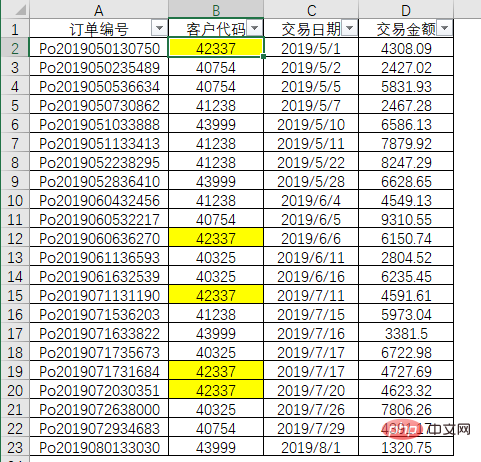
In fact, it is very convenient to use formulas to count the number of unique data. For example, in the situation below, you need to count the number of unique customers:
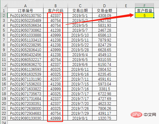
Usually there are two formulas for counting the number of unique data. Today I will share with you the principle of the first formula.
Routine 1: Combination of SUMPRODUCT and COUNTIF
First let’s take a look at the formula input process:
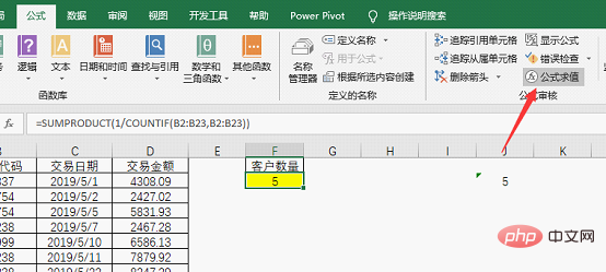
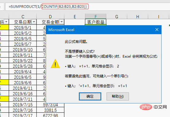
The operation is not difficult, but the difficulty is that many people do not understand the principle of the formula =SUMPRODUCT(1/COUNTIF(B2:B23,B2:B23)).
I understand each function individually, but when combined together I feel confused. I believe this is the feeling shared by many beginners. In fact, it is not as difficult to understand the principle of this formula as everyone thinks. As long as you can use a tool called formula evaluation and a function key called F9, you can crack the secret of the formula. The specific process will be introduced below.
Select the cell where the formula is located and click the Evaluate Formula button.
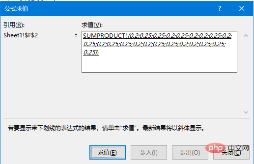
The usage of this function is very simple, as shown in the figure:
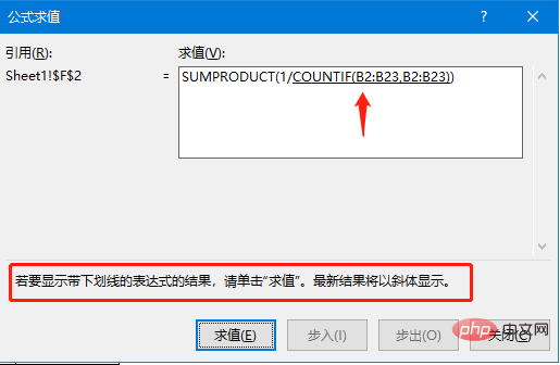
The underlined part indicates that it will be displayed soon. As for the location of the results, you can see from the picture that the first thing to calculate is the COUNTIF(B2:B23,B2:B23) part. Click "Evaluate" to see what results you can get.

We got a set of numbers that represent the number of times each customer code appears. For example, the first 5 means that customer 42337 appears five times. This is also COUNTIF The most basic functionality.
Continue to click "Evaluate" and you can see the results of 1/COUNTIF, as shown in the figure:
After using F9 to display the results, you can click ✖ on the left side of the editing bar, or press the Esc key to exit. If you accidentally press Enter, you can use Undo or the Ctrl Z key combination to return to the original formula.
Routine 2: Combination of COUNT and MATCH
This formula is a little more difficult, let’s take a look at the operation process.
This formula is an array formula. Remember to press Ctrl Shift and Enter after completing the input. Braces will automatically appear on both sides of the formula.
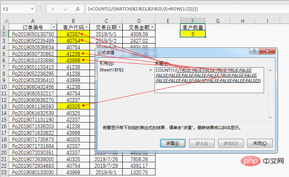
Formula=COUNT(1/(MATCH(B2:B23,B2:B23,0)=ROW(1:22)))Three functions are used, COUNT, MATCH and ROW, regardless of operation or principle, this formula is more difficult than the first formula.
So why do we need to introduce this formula?
This is because some of the ideas and methods used in this formula will be encountered repeatedly in many powerful formulas. Therefore, understanding the second routine will help improve the ability to use the formula.
Getting back to the topic, let’s use formula evaluation to crack the principle of this formula.

Simply speaking, MATCH has three parameters, search value, search area and search method. What the formula obtains is the position where the search value first appears in the search area. Click to find value to see the result.
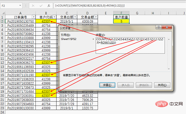
Let’s look at customer 42337, which appears five times in total. The results obtained by the MATCH function are all 1, indicating that the position where this customer first appeared is 1.
It should be emphasized that this 1 is the position in the search range, and our search range starts from the second line.
For this set of data obtained by MATCH, you must understand its meaning. Continue point evaluation to get the result of this part of ROW.
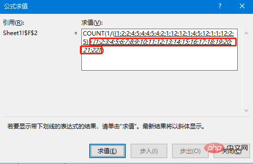
ROW can get the row number corresponding to the parameter. For example, ROW(A1), the result is 1, and ROW(1:22), the result is the first 22 rows. Number, that is, the group of numbers 1 to 22.
Note that the range in the formula MATCH(B2:B23,B2:B23,0)=ROW(1:22) is different. MATCH is from 2 to 23 rows, which is actually 22 rows of data, while ROW The range is based on the actual number of rows of data.
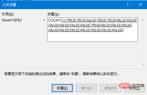
Continue to evaluate. The formula will determine whether the set of data obtained by MATCH is consistent with the set of data obtained by ROW. The result is a set of logical values.
It can be found from the results that the formula result is TRUE at the position where each customer first appears.
It is necessary to popularize the knowledge of logical values here.
There are six comparison symbols in Excel, = (equal to), > (greater than), (less than), >= (greater than or equal to), (less than or equal to), (not equal to) , equal to is used in this example.
The result of the comparison is a logical value. There are two logical values, TRUE and FALSE. TRUE means the result is correct, and FALSE means the result is incorrect.
For example, 1>2, the result of this comparison is FALSE.
When logical values are used for addition, subtraction, multiplication, and division with numbers, TRUE is equivalent to 1, and FALSE is equivalent to 0.
In this step of calculation, the number 1 and this set of logical values are used for calculation. When the denominator is TRUE, 1/1 gets 1; when the denominator is FALSE When 1/0 will get the wrong value, the denominator is zero.
Click evaluate to see the result.
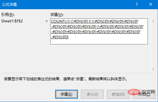
If you understand the above principles, the final result will be easy to understand.
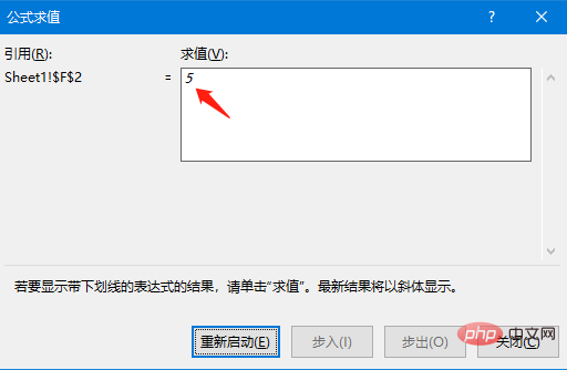
Because COUNT only does one thing, counting several numbers. In this set of results, only five 1's are numbers, so the final result is 5.
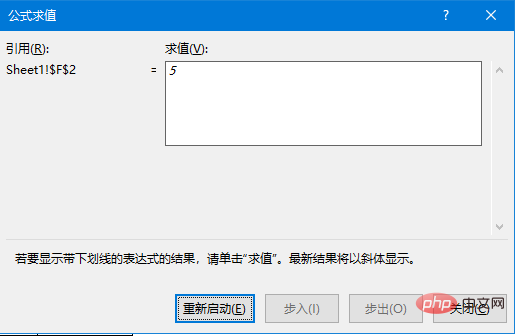
Many times, 1/ is replaced by 0/. Maybe this is a habit of experts.
When you truly understand the principles of the formula, 1/ and 0/ will no longer be the cause of your troubles.
This concludes the analysis of the principle of the second formula. In this formula, many common skills used in advanced formulas are used, such as using ROW to obtain an array, and using various comparison operations to obtain a set of logical values. , and then obtain some error values through calculation of logical values (error values are not useless at all). There is no difference in most cases except for some special cases whether to use 0/ or 1/.
Okay, the analysis of the two formulas for counting the number of non-duplicate data has come to an end. If you still encounter any formulas that cannot be cracked, you can leave a message and tell the editor, and we will figure it out together.
Related learning recommendations: excel tutorial
The above is the detailed content of Practical Excel skills sharing: Two magical skills will help you see the secret of counting unique numbers!. For more information, please follow other related articles on the PHP Chinese website!

Hot AI Tools

Undresser.AI Undress
AI-powered app for creating realistic nude photos

AI Clothes Remover
Online AI tool for removing clothes from photos.

Undress AI Tool
Undress images for free

Clothoff.io
AI clothes remover

AI Hentai Generator
Generate AI Hentai for free.

Hot Article
Hot Tools

Notepad++7.3.1
Easy-to-use and free code editor

SublimeText3 Chinese version
Chinese version, very easy to use

Zend Studio 13.0.1
Powerful PHP integrated development environment

Dreamweaver CS6
Visual web development tools

SublimeText3 Mac version
God-level code editing software (SublimeText3)
Hot Topics
 1376
1376
 52
52

 What should I do if the frame line disappears when printing in Excel?
Mar 21, 2024 am 09:50 AM
What should I do if the frame line disappears when printing in Excel?
Mar 21, 2024 am 09:50 AM
If when opening a file that needs to be printed, we will find that the table frame line has disappeared for some reason in the print preview. When encountering such a situation, we must deal with it in time. If this also appears in your print file If you have questions like this, then join the editor to learn the following course: What should I do if the frame line disappears when printing a table in Excel? 1. Open a file that needs to be printed, as shown in the figure below. 2. Select all required content areas, as shown in the figure below. 3. Right-click the mouse and select the "Format Cells" option, as shown in the figure below. 4. Click the “Border” option at the top of the window, as shown in the figure below. 5. Select the thin solid line pattern in the line style on the left, as shown in the figure below. 6. Select "Outer Border"
 How to filter more than 3 keywords at the same time in excel
Mar 21, 2024 pm 03:16 PM
How to filter more than 3 keywords at the same time in excel
Mar 21, 2024 pm 03:16 PM
Excel is often used to process data in daily office work, and it is often necessary to use the "filter" function. When we choose to perform "filtering" in Excel, we can only filter up to two conditions for the same column. So, do you know how to filter more than 3 keywords at the same time in Excel? Next, let me demonstrate it to you. The first method is to gradually add the conditions to the filter. If you want to filter out three qualifying details at the same time, you first need to filter out one of them step by step. At the beginning, you can first filter out employees with the surname "Wang" based on the conditions. Then click [OK], and then check [Add current selection to filter] in the filter results. The steps are as follows. Similarly, perform filtering separately again
 How to change excel table compatibility mode to normal mode
Mar 20, 2024 pm 08:01 PM
How to change excel table compatibility mode to normal mode
Mar 20, 2024 pm 08:01 PM
In our daily work and study, we copy Excel files from others, open them to add content or re-edit them, and then save them. Sometimes a compatibility check dialog box will appear, which is very troublesome. I don’t know Excel software. , can it be changed to normal mode? So below, the editor will bring you detailed steps to solve this problem, let us learn together. Finally, be sure to remember to save it. 1. Open a worksheet and display an additional compatibility mode in the name of the worksheet, as shown in the figure. 2. In this worksheet, after modifying the content and saving it, the dialog box of the compatibility checker always pops up. It is very troublesome to see this page, as shown in the figure. 3. Click the Office button, click Save As, and then
 How to type subscript in excel
Mar 20, 2024 am 11:31 AM
How to type subscript in excel
Mar 20, 2024 am 11:31 AM
eWe often use Excel to make some data tables and the like. Sometimes when entering parameter values, we need to superscript or subscript a certain number. For example, mathematical formulas are often used. So how do you type the subscript in Excel? ?Let’s take a look at the detailed steps: 1. Superscript method: 1. First, enter a3 (3 is superscript) in Excel. 2. Select the number "3", right-click and select "Format Cells". 3. Click "Superscript" and then "OK". 4. Look, the effect is like this. 2. Subscript method: 1. Similar to the superscript setting method, enter "ln310" (3 is the subscript) in the cell, select the number "3", right-click and select "Format Cells". 2. Check "Subscript" and click "OK"
 How to set superscript in excel
Mar 20, 2024 pm 04:30 PM
How to set superscript in excel
Mar 20, 2024 pm 04:30 PM
When processing data, sometimes we encounter data that contains various symbols such as multiples, temperatures, etc. Do you know how to set superscripts in Excel? When we use Excel to process data, if we do not set superscripts, it will make it more troublesome to enter a lot of our data. Today, the editor will bring you the specific setting method of excel superscript. 1. First, let us open the Microsoft Office Excel document on the desktop and select the text that needs to be modified into superscript, as shown in the figure. 2. Then, right-click and select the "Format Cells" option in the menu that appears after clicking, as shown in the figure. 3. Next, in the “Format Cells” dialog box that pops up automatically
 How to use the iif function in excel
Mar 20, 2024 pm 06:10 PM
How to use the iif function in excel
Mar 20, 2024 pm 06:10 PM
Most users use Excel to process table data. In fact, Excel also has a VBA program. Apart from experts, not many users have used this function. The iif function is often used when writing in VBA. It is actually the same as if The functions of the functions are similar. Let me introduce to you the usage of the iif function. There are iif functions in SQL statements and VBA code in Excel. The iif function is similar to the IF function in the excel worksheet. It performs true and false value judgment and returns different results based on the logically calculated true and false values. IF function usage is (condition, yes, no). IF statement and IIF function in VBA. The former IF statement is a control statement that can execute different statements according to conditions. The latter
 Where to set excel reading mode
Mar 21, 2024 am 08:40 AM
Where to set excel reading mode
Mar 21, 2024 am 08:40 AM
In the study of software, we are accustomed to using excel, not only because it is convenient, but also because it can meet a variety of formats needed in actual work, and excel is very flexible to use, and there is a mode that is convenient for reading. Today I brought For everyone: where to set the excel reading mode. 1. Turn on the computer, then open the Excel application and find the target data. 2. There are two ways to set the reading mode in Excel. The first one: In Excel, there are a large number of convenient processing methods distributed in the Excel layout. In the lower right corner of Excel, there is a shortcut to set the reading mode. Find the pattern of the cross mark and click it to enter the reading mode. There is a small three-dimensional mark on the right side of the cross mark.
 How to insert excel icons into PPT slides
Mar 26, 2024 pm 05:40 PM
How to insert excel icons into PPT slides
Mar 26, 2024 pm 05:40 PM
1. Open the PPT and turn the page to the page where you need to insert the excel icon. Click the Insert tab. 2. Click [Object]. 3. The following dialog box will pop up. 4. Click [Create from file] and click [Browse]. 5. Select the excel table to be inserted. 6. Click OK and the following page will pop up. 7. Check [Show as icon]. 8. Click OK.
