
 Technology peripherals
AI
Decision-making positioning application based on causal forest algorithm
Technology peripherals
AI
Decision-making positioning application based on causal forest algorithm
Decision-making positioning application based on causal forest algorithm

Translator | Zhu Xianzhong
Reviewer|Sun Shujuan
In my previous blog, we have explainedhow to use causal trees to evaluate policy heterogeneity HandlingEffect. If you haven't read, I suggest you read it before reading this article, because weIn this articleI thinkYou have understood the part of the in this article and the content related to this article.
Why are heterogenous treatment effects (HTE: heterogenous treatment effects) ? First, the estimation of heterogeneous treatment effects allows us to condition their on their expected outcomes (illness, firm revenue, customer satisfaction etc.) Users (patients, users, customers, etc.) who choose to provide processing (drugs, advertisements, products, etc.). In other words, it is estimated that HTE helps us in targeting. In fact, as we will see later in the article, one processing method is bringing positive results to some users. While beneficial, it may be ineffective or even counterproductive on average. The opposite may also be true: A drug is effective on average, but isif weare clearIt has side effects for usersIf the information#the effectiveness of this drugwillFurther improve.
#In this article, we will explore an extension of the causal tree - the causalforest forest. Just as random forests expand regression trees by averaging multiple bootstrap trees together, causal forests also expand causal trees. The main difference comes from the reasoning perspective, which is less straightforward. We will also see how the outputs of different HTE estimation algorithms can be compared and how they can be used for policy objectives. Online Discount Case
In the rest of this article, we continue to useMy last article about Toy example used in the Cause and Effect Tree article: Let’s assume we are an online store and we are interested in knowing whether offering discounts to new customers will increase their spending in the store.
To understand whether the discount is a good deal, we conducted the following randomized experiment, or A/B test: Every time a new customer browses our online store, we randomly assign them to a treatment condition. We offer discounts to users who are processed; and we do not offer discounts to users who are in control. I import the data generation process dgp_online_discounts() from filesrc.dgp. I also import some drawing functions and libraries from src.utilslibraries. In order to include not only code, but also data and tables, I used the Deepnote framework, which is a Jupyter-based Web's collaborative notebook environment.
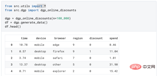
observewhether they got a discount, how we handled it, how much they spent, and some other interesting results.
Since theexperiment is randomly assigned, we can use a simple mean difference estimate to estimate ExperimentEffect. We expect the experiment and control groups to be similar except for the discount, so we can attribute any differences in spending to the discount.
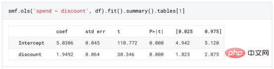
Looks like seems to be valid:ExperimentThe average spend increased by $1.95. But are all customers affected equally?
To answer this question, we would like to estimate the heterogeneoustreatmenteffect, Probably on an individual level. Causal Forest
CalculateHeterogeneous treatment effectsThere are many different options . The simplest approach is to interact with the outcome of interest in terms of heterogeneity dimensions. The problem with this approach is which variable to choose. Sometimes, we have information that may guide our actions in advance; for example, we may know that mobile users spend more on average than desktop users many. Other times, we may be interested in a certain dimension for commercial reasons; for example, we may want to invest more in a certain region. However, when we have no additional information, we want the process to be data-driven. In a previous article, we explored a data-driven approach to estimating heterogeneous treatment effects
——Causal tree. We will now extend them to causal forests. However, before we begin, we must introduce its non-causal cousin, the random forest.
Random forest, as the name suggests, is an extension of the regression tree, adding two independent sources of randomness to it. In particular, the random forest algorithm is able to make predictions on many different regression trees, each on a bootstrap sample Do the training and average them together. This process is often called the guided aggregation algorithm, also known as the bagging algorithm, and can be applied to any prediction algorithm and is not specific to random forests. An additional source of randomness comes from feature selection, since at each split only a random subset of all features X are considered for the optimal split.
#These two additional sources of randomness are very important and help improve the performance of random forests. First, the bagging algorithm allows random forests to produce smoother predictions than regression trees by averaging multiple discrete predictions. In contrast, random feature selection allows random forests to explore the feature space more deeply, allowing them to discover more interactions than simple regression trees. In fact, there may be interactions between variables that are not very predictive on their own (and therefore not divisive), but are very powerful together.
Causal forest is equivalent to random forest, but used to estimate heterogeneous treatment effects, unlike causal trees It is exactly the same as regression tree. As with causal trees, we have a basic problem: we are interested in predicting an object that we have not observed: the individual treatmenteffectτᵢ. The solution is to create an auxiliary result variable Y* whose expected value for each observation is exactly the processing effect.
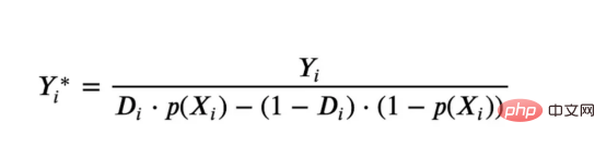
Auxiliary result variable
If you want to understand morewhy this variable has no effect on the individualtreatmentadding bias, please take a look at My previous article, I am here## A detailed introduction is given in # articles. In short, you canthinkYᵢ* as an estimator of the mean difference for a single observation. Once we have an outcome variable, there are a few more things we need to do in order to use random forests to estimate heterogeneous treatment effects
. First, we need to build the tree with the same number of processing units and control units on each leaf. Secondly, we need to use different samples to build the tree and evaluate it, i.e. calculate the average result for each leaf. This process is often called honest trees because we can treat the samples of each leaf as independent of the tree structure, so it is very useful for inference. Before proceeding with the evaluation, let us first generate dummy variables for the categorical variables device, browser and
region .
1 2 3 |
|
. Fortunately, we don't have to do all of this manually, because is already available in Microsoft's EconML package Provides a good causal tree and forest implementation. We will use the CausalForestML function from .
1 2 3 4 5 |
|
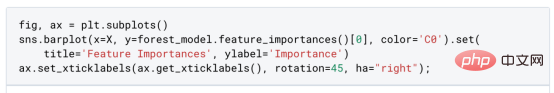
与因果树不同,因果森林更难解释,因为我们无法可视化每一棵树。我们可以使用SingleTreeateInterpreter函数来绘制因果森林算法的等效表示。
1 2 3 4 |
|
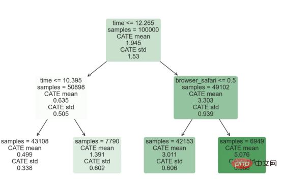
因果森林模型表示
我们可以像因果树模型一样解释树形图。在顶部,我们可以看到数据中的平均$Y^*$的值为1.917$。从那里开始,根据每个节点顶部突出显示的规则,数据被拆分为不同的分支。例如,根据时间是否晚于11.295,第一节点将数据分成大小为46878$和53122$的两组。在底部,我们得到了带有预测值的最终分区。例如,最左边的叶子包含40191$的观察值(时间早于11.295,在非Safari浏览器环境下),我们预测其花费为0.264$。较深的节点颜色表示预测值较高。
这种表示的问题在于,与因果树的情况不同,它只是对模型的解释。由于因果森林是由许多自助树组成的,因此无法直接检查每个决策树。了解在确定树分割时哪个特征最重要的一种方法是所谓的特征重要性。
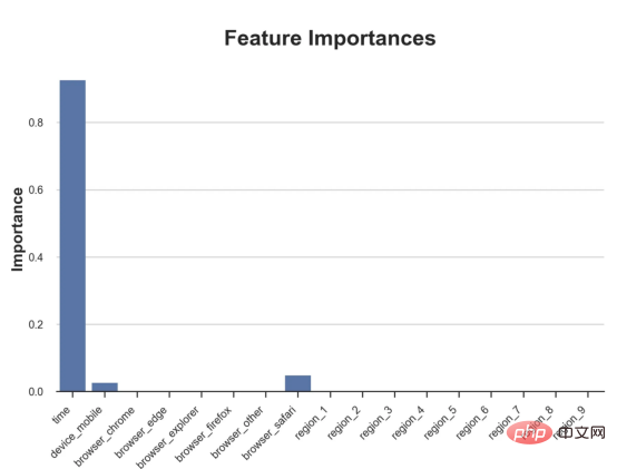
显然,时间是异质性的第一个维度,其次是设备(特别是移动设备)和浏览器(特别是Safari)。其他维度无关紧要。
现在,让我们检查一下模型性能如何。
性能
通常,我们无法直接评估模型性能,因为与标准的机器学习设置不同,我们没有观察到实际情况。因此,我们不能使用测试集来计算模型精度的度量。然而,在我们的案例中,我们控制了数据生成过程,因此我们可以获得基本的真相。让我们从分析模型如何沿着数据、设备、浏览器和区域的分类维度估计异质处理效应开始。
1 2 3 4 5 6 7 8 9 10 11 12 13 14 15 |
|
对于每个分类变量,我们绘制了实际和估计的平均处理效果。
1 2 3 4 |
|
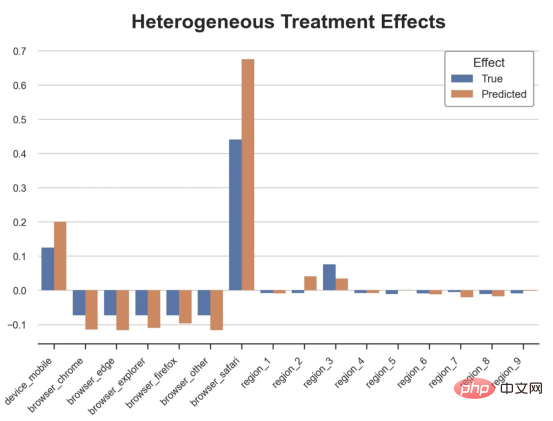
作者提供的每个分类值的真实和估计处理效果
因果森林算法非常善于预测与分类变量相关的处理效果。至于因果树,这是预期的,因为算法具有非常离散的性质。然而,与因果树不同的是,预测更加微妙。
我们现在可以做一个更相关的测试:算法在时间等连续变量下的表现如何?首先,让我们再次隔离预测的处理效果,并忽略其他协变量。
def compute_time_effect(df, hte_model, avg_effect_notime):
1 2 3 4 5 6 7 |
|
我们现在可以复制之前的数字,但时间维度除外。我们绘制了一天中每个时间的平均真实和估计处理效果。
1 2 3 4 |
|
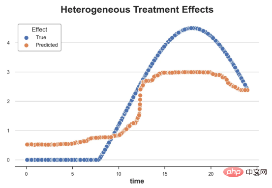
沿时间维度绘制的真实和估计的处理效果
我们现在可以充分理解因果树和森林之间的区别:虽然在因果树的情况下,估计基本上是一个非常粗略的阶跃函数,但我们现在可以看到因果树如何产生更平滑的估计。
我们现在已经探索了该模型,是时候使用它了!
策略定位
假设我们正在考虑向访问我们在线商店的新客户提供4美元的折扣。
1 |
|
折扣对哪些客户有效?我们估计平均处理效果为1.9492美元。这意味着,平均而言折扣并不真正有利可图。然而,现在可以针对单个客户,我们只能向一部分新客户提供折扣。我们现在将探讨如何进行政策目标定位,为了更好地了解目标定位的质量,我们将使用因果树模型作为参考点。
我们使用相同的CauselForestML函数构建因果树,但将估计数和森林大小限制为1。
1 2 3 4 5 |
|
接下来,我们将数据集分成一个训练集和一个测试集。这一想法与交叉验证非常相似:我们使用训练集来训练模型——在我们的案例中是异质处理效应的估计器——并使用测试集来评估其质量。主要区别在于,我们没有观察到测试数据集中的真实结果。但是我们仍然可以使用训练测试分割来比较样本内预测和样本外预测。
我们将所有观察结果的80%放在训练集中,20%放在测试集中。
1 |
|
首先,让我们仅在训练样本上重新训练模型。
1 2 3 |
|
现在,我们可以确定目标策略,即决定我们向哪些客户提供折扣。答案似乎很简单:我们向所有预期处理效果大于成本(4美元)的客户提供折扣。
借助于一个可视化工具,它可以让我们了解处理对谁有效以及如何有效,这就是所谓的处理操作特征(TOC)曲线。这个名字可以看作是基于另一个更著名的接收器操作特性(ROC)曲线的修正,该曲线描绘了二元分类器的不同阈值的真阳性率与假阳性率。这两种曲线的想法类似:我们绘制不同比例受处理人群的平均处理效果。在一个极端情况下,当所有客户都被处理时,曲线的值等于平均处理效果;而在另一个极端情况下,当只有一个客户被处理时曲线的值则等于最大处理效果。
现在让我们计算曲线。
1 2 3 4 5 6 7 8 9 10 11 12 13 14 15 |
|
现在,我们可以绘制两个CATE估算器的处理操作特征(TOC)曲线。
1 2 3 4 5 6 7 8 9 10 11 12 13 14 15 |
|
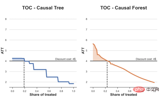
处理操作特性曲线
正如预期的那样,两种估算器的TOC曲线都在下降,因为平均效应随着我们处理客户份额的增加而降低。换言之,我们在发布折扣时越有选择,每个客户的优惠券效果就越高。我还画了一条带有折扣成本的水平线,以便我们可以将TOC曲线下方和成本线上方的阴影区域解释为预期利润。
这两种算法预测的处理份额相似,约为20%,因果森林算法针对的客户略多一些。然而,他们预测的利润结果却大相径庭。因果树算法预测的边际较小且恒定,而因果林算法预测的是更大且更陡的边际。那么,哪一种算法更准确呢?
为了比较它们,我们可以在测试集中对它们进行评估。我们采用训练集上训练的模型,预测处理效果,并将其与测试集上训练模型的预测进行比较。注意,与机器学习标准测试程序不同,有一个实质性的区别:在我们的案例中,我们无法根据实际情况评估我们的预测,因为没有观察到处理效果。我们只能将两个预测相互比较。
1 2 3 4 5 6 7 8 9 10 11 12 13 14 15 16 17 18 19 20 |
|
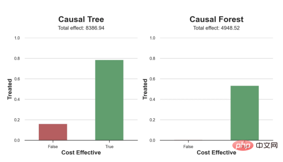
因果树模型似乎比因果森林模型表现得更好一些,总净效应为8386美元——相对于4948美元。从图中,我们也可以了解差异的来源。因果森林算法往往限制性更强,处理的客户更少,没有误报的阳性,但也有很多误报的阴性。另一方面,因果树算法看起来更加“慷慨”,并将折扣分配给更多的新客户。这既转化为更多的真阳性,也转化为假阳性。总之,净效应似乎有利于因果树算法。
通常,我们讨论到这里就可以停止了,因为我们可以做的事情不多了。然而,在我们的案例情形中,我们还可以访问真正的数据生成过程。因此,接下来我们不妨检查一下这两种算法的真实精度。
首先,让我们根据处理效果的预测误差来比较它们。对于每个算法,我们计算处理效果的均方误差。
1 2 3 4 5 6 7 8 9 |
|
结果是,随机森林模型更好地预测了平均处理效果,均方误差为0.5555美元,而不是0.9035美元。
那么,这是否意味着更好的目标定位呢?我们现在可以复制上面所做的相同的柱状图,以了解这两种算法在策略目标方面的表现。
1 2 3 |
|
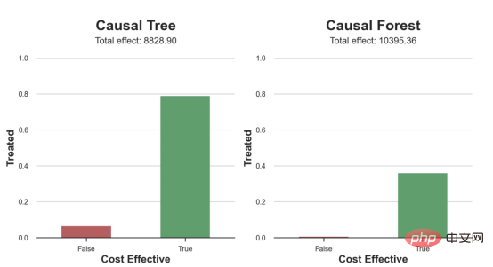
这两幅图非常相似,但结果却大相径庭。事实上,因果森林算法现在优于因果树算法,总效果为10395美元,而非8828美元。为什么会出现这种突然的差异呢?
为了更好地理解差异的来源,让我们根据实际情况绘制TOC。
1 2 3 4 |
|
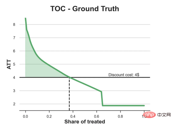
处理操作特性曲线。
正如我们所看到的,TOC是倾斜度非常大的,存在一些平均处理效果非常高的客户。随机森林算法能够更好地识别它们,因此总体上更有效,尽管目标客户较少些。
Conclusion
In this article, we learned a functionvery Powerful #algorithms for estimating heterogeneous treatment effects - causal forests. Causal forests are built on the same principles as causal trees, but benefit from a deeper exploration of parameter space and bagging algorithms.
In addition,we alsolearnedhow to useEstimation of heterogeneous treatment effects to implement policypositioning. By identifying users with the highest processing effectiveness, we are able to ensure that a policy is profitable. We also see that the policy objectives differ from the heterogeneous treatment effects assessment objectives, as the tails of the distribution may have stronger # than the mean ##Correlation.
References- S. Athey, G. Imbens, Recursive partitioning for heterogeneous causal effects (2016), PNAS .
- S. Wager, S. Athey, Estimation and Inference of Heterogeneous Treatment Effects using Random Forests (2018), Journal of the American Statistical Association.
- S. Athey, J. Tibshirani, S. Wager, Generalized Random Forests (2019). The Annals of Statistics.
- M. Oprescu, V. Syrgkanis, Z. Wu, Orthogonal Random Forest for Causal Inference (2019). Proceedings of the 36th International Conference on Machine Learning.
Zhu Xianzhong, 51CTO community editor, 51CTO expert blogger, lecturer, Weifang No.1 A computer teacher in a university and a veteran in the field of freelance programming.
Original title: From Causal Trees to Forests, by Matteo Courthoud
The above is the detailed content of Decision-making positioning application based on causal forest algorithm. For more information, please follow other related articles on the PHP Chinese website!

Hot AI Tools

Undresser.AI Undress
AI-powered app for creating realistic nude photos

AI Clothes Remover
Online AI tool for removing clothes from photos.

Undress AI Tool
Undress images for free

Clothoff.io
AI clothes remover

AI Hentai Generator
Generate AI Hentai for free.
Hot Article
Hot Tools

Notepad++7.3.1
Easy-to-use and free code editor

SublimeText3 Chinese version
Chinese version, very easy to use

Zend Studio 13.0.1
Powerful PHP integrated development environment

Dreamweaver CS6
Visual web development tools

SublimeText3 Mac version
God-level code editing software (SublimeText3)
Hot Topics
 1386
1386
 52
52

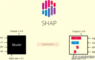 This article will take you to understand SHAP: model explanation for machine learning
Jun 01, 2024 am 10:58 AM
This article will take you to understand SHAP: model explanation for machine learning
Jun 01, 2024 am 10:58 AM
In the fields of machine learning and data science, model interpretability has always been a focus of researchers and practitioners. With the widespread application of complex models such as deep learning and ensemble methods, understanding the model's decision-making process has become particularly important. Explainable AI|XAI helps build trust and confidence in machine learning models by increasing the transparency of the model. Improving model transparency can be achieved through methods such as the widespread use of multiple complex models, as well as the decision-making processes used to explain the models. These methods include feature importance analysis, model prediction interval estimation, local interpretability algorithms, etc. Feature importance analysis can explain the decision-making process of a model by evaluating the degree of influence of the model on the input features. Model prediction interval estimate
 Implementing Machine Learning Algorithms in C++: Common Challenges and Solutions
Jun 03, 2024 pm 01:25 PM
Implementing Machine Learning Algorithms in C++: Common Challenges and Solutions
Jun 03, 2024 pm 01:25 PM
Common challenges faced by machine learning algorithms in C++ include memory management, multi-threading, performance optimization, and maintainability. Solutions include using smart pointers, modern threading libraries, SIMD instructions and third-party libraries, as well as following coding style guidelines and using automation tools. Practical cases show how to use the Eigen library to implement linear regression algorithms, effectively manage memory and use high-performance matrix operations.
 Five schools of machine learning you don't know about
Jun 05, 2024 pm 08:51 PM
Five schools of machine learning you don't know about
Jun 05, 2024 pm 08:51 PM
Machine learning is an important branch of artificial intelligence that gives computers the ability to learn from data and improve their capabilities without being explicitly programmed. Machine learning has a wide range of applications in various fields, from image recognition and natural language processing to recommendation systems and fraud detection, and it is changing the way we live. There are many different methods and theories in the field of machine learning, among which the five most influential methods are called the "Five Schools of Machine Learning". The five major schools are the symbolic school, the connectionist school, the evolutionary school, the Bayesian school and the analogy school. 1. Symbolism, also known as symbolism, emphasizes the use of symbols for logical reasoning and expression of knowledge. This school of thought believes that learning is a process of reverse deduction, through existing
 Explainable AI: Explaining complex AI/ML models
Jun 03, 2024 pm 10:08 PM
Explainable AI: Explaining complex AI/ML models
Jun 03, 2024 pm 10:08 PM
Translator | Reviewed by Li Rui | Chonglou Artificial intelligence (AI) and machine learning (ML) models are becoming increasingly complex today, and the output produced by these models is a black box – unable to be explained to stakeholders. Explainable AI (XAI) aims to solve this problem by enabling stakeholders to understand how these models work, ensuring they understand how these models actually make decisions, and ensuring transparency in AI systems, Trust and accountability to address this issue. This article explores various explainable artificial intelligence (XAI) techniques to illustrate their underlying principles. Several reasons why explainable AI is crucial Trust and transparency: For AI systems to be widely accepted and trusted, users need to understand how decisions are made
 Is Flash Attention stable? Meta and Harvard found that their model weight deviations fluctuated by orders of magnitude
May 30, 2024 pm 01:24 PM
Is Flash Attention stable? Meta and Harvard found that their model weight deviations fluctuated by orders of magnitude
May 30, 2024 pm 01:24 PM
MetaFAIR teamed up with Harvard to provide a new research framework for optimizing the data bias generated when large-scale machine learning is performed. It is known that the training of large language models often takes months and uses hundreds or even thousands of GPUs. Taking the LLaMA270B model as an example, its training requires a total of 1,720,320 GPU hours. Training large models presents unique systemic challenges due to the scale and complexity of these workloads. Recently, many institutions have reported instability in the training process when training SOTA generative AI models. They usually appear in the form of loss spikes. For example, Google's PaLM model experienced up to 20 loss spikes during the training process. Numerical bias is the root cause of this training inaccuracy,
 Improved detection algorithm: for target detection in high-resolution optical remote sensing images
Jun 06, 2024 pm 12:33 PM
Improved detection algorithm: for target detection in high-resolution optical remote sensing images
Jun 06, 2024 pm 12:33 PM
01 Outlook Summary Currently, it is difficult to achieve an appropriate balance between detection efficiency and detection results. We have developed an enhanced YOLOv5 algorithm for target detection in high-resolution optical remote sensing images, using multi-layer feature pyramids, multi-detection head strategies and hybrid attention modules to improve the effect of the target detection network in optical remote sensing images. According to the SIMD data set, the mAP of the new algorithm is 2.2% better than YOLOv5 and 8.48% better than YOLOX, achieving a better balance between detection results and speed. 02 Background & Motivation With the rapid development of remote sensing technology, high-resolution optical remote sensing images have been used to describe many objects on the earth’s surface, including aircraft, cars, buildings, etc. Object detection in the interpretation of remote sensing images
 Machine Learning in C++: A Guide to Implementing Common Machine Learning Algorithms in C++
Jun 03, 2024 pm 07:33 PM
Machine Learning in C++: A Guide to Implementing Common Machine Learning Algorithms in C++
Jun 03, 2024 pm 07:33 PM
In C++, the implementation of machine learning algorithms includes: Linear regression: used to predict continuous variables. The steps include loading data, calculating weights and biases, updating parameters and prediction. Logistic regression: used to predict discrete variables. The process is similar to linear regression, but uses the sigmoid function for prediction. Support Vector Machine: A powerful classification and regression algorithm that involves computing support vectors and predicting labels.
 Outlook on future trends of Golang technology in machine learning
May 08, 2024 am 10:15 AM
Outlook on future trends of Golang technology in machine learning
May 08, 2024 am 10:15 AM
The application potential of Go language in the field of machine learning is huge. Its advantages are: Concurrency: It supports parallel programming and is suitable for computationally intensive operations in machine learning tasks. Efficiency: The garbage collector and language features ensure that the code is efficient, even when processing large data sets. Ease of use: The syntax is concise, making it easy to learn and write machine learning applications.
