Image classification with few-shot learning using PyTorch
In recent years, deep learning-based models have performed well in tasks such as target detection and image recognition. On challenging image classification datasets like ImageNet, which contains 1,000 different object classifications, some models now exceed human levels. But these models rely on a supervised training process, they are significantly affected by the availability of labeled training data, and the classes the models are able to detect are limited to the classes they were trained on.
Since there are not enough labeled images for all classes during training, these models may be less useful in real-world settings. And we want the model to be able to recognize classes it has not seen during training, since it is almost impossible to train on images of all potential objects. The problem where we will learn from a few samples is called Few-Shot learning.
What is few-shot learning?

Few-shot learning is a subfield of machine learning. It involves classifying new data with only a few training samples and supervision data. The model we created performs reasonably well with only a small number of training samples.
Consider the following scenario: In the medical field, for some uncommon diseases, there may not be enough x-ray images for training. For such scenarios, building a few-shot learning classifier is the perfect solution.
Changes in Small Samples
Generally speaking, researchers have identified four types:
- N-Shot Learning (NSL)
- Few-Shot Learning (FSL)
- One-Shot Learning (OSL)
- Zero-Shot Learning (ZSL)
When we talk about FSL, we usually Refers to the N-way-K-Shot classification. N represents the number of classes, and K represents the number of samples to be trained in each class. So N-Shot Learning is considered as a broader concept than all other concepts. It can be said that Few-Shot, One-Shot and Zero-Shot are sub-fields of NSL. While zero-shot learning aims to classify unseen classes without any training examples.
In One-Shot Learning, there is only one sample for each class. Few-Shot has 2 to 5 samples per class, which means Few-Shot is a more flexible version of One-Shot Learning.
Small sample learning method
Generally, two methods should be considered when solving the Few Shot Learning problem:
Data Level Approach (DLA)
This The strategy is very simple, if there is not enough data to create a solid model and prevent underfitting and overfitting, then more data should be added. Because of this, many FSL problems can be solved by leveraging more data from a larger underlying data set. A notable feature of the base dataset is that it lacks the classes that constitute our support set for the Few-Shot challenge. For example, if we want to classify a certain species of bird, the underlying data set may contain pictures of many other birds.
Parameter-level approach (PLA)
From a parameter-level perspective, Few-Shot Learning samples are relatively easy to overfit because they usually have large high-dimensional spaces. Restricting the parameter space, using regularization and using an appropriate loss function will help solve this problem. A small number of training samples will be used by the model to generalize.
Performance can be improved by guiding the model into a broad parameter space. Normal optimization methods may not produce accurate results due to lack of training data.
For the reasons above, training our model to find the best path through the parameter space produces the best prediction results. This approach is called meta-learning.
Small sample learning image classification algorithm
There are 4 common small sample learning methods:
Model-independent meta-learning Model-Agnostic Meta-Learning
The gradient-based meta-learning (GBML) principle is the basis of MAML. In GBML, meta-learners gain prior experience by training on a base model and learning shared features across all task representations. Each time there is a new task to learn, the meta-learner is fine-tuned using its existing experience and the minimum amount of new training data provided by the new task.
Generally, if we randomly initialize parameters and update them several times, the algorithm will not converge to good performance. MAML attempts to solve this problem. MAML provides a reliable initialization of the meta-parameter learner with only a few gradient steps and guarantees no overfitting, so that new tasks can be optimally and quickly learned.
The steps are as follows:
- The meta-learner creates its own copy C at the beginning of each episode,
- C is trained on this episode (With the help of base-model),
- C makes predictions on the query set,
- The loss calculated from these predictions is used to update C,
- This This continues until all episodes of training are completed.
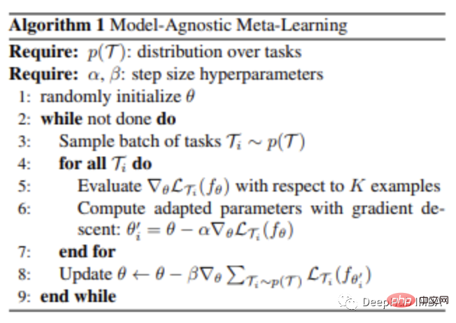
The biggest advantage of this technique is that it is considered independent of the choice of meta-learning algorithm. Therefore, MAML methods are widely used in many machine learning algorithms that require rapid adaptation, especially deep neural networks.
Matching Networks
The first metric learning method created to solve the FSL problem was the Matching Network (MN).
A large base data set is required when using the matching network method to solve the Few-Shot Learning problem. .
After dividing the dataset into several episodes, for each episode, the matching network does the following:
- Every image from the support set and the query set is fed to a CNN that outputs embeddings of features for them
- Query images using a model trained on the support set to get the cosine distance of the embedded features, classify by softmax
- Cross entropy loss for classification results by CNN Backpropagation Update Feature Embedding Model
The matching network can learn to build image embeddings in this way. MN is able to classify photos using this method without any special prior knowledge of the categories. He simply compares several instances of the class.
Because categories vary from episode to episode, the matching network computes image attributes (features) that are important for category distinction. When using standard classification, the algorithm selects features that are unique to each category.
Prototypical Networks
Similar to the matching network is the prototype network (PN). It improves the performance of the algorithm through some subtle changes. PN achieves better results than MN, but their training process is essentially the same, just comparing some query image embeddings from the support set, but the prototype network provides different strategies.
We need to create a prototype of the class in PN: the embedding of the class created by averaging the embeddings of the images in the class. Then only these class prototypes are used to compare query image embeddings. When used for single-sample learning problems, it is comparable to matching networks.
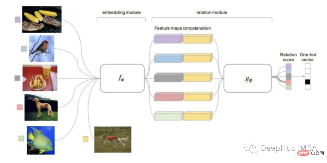
Relation Network Relation Network
Relationship network can be said to have inherited the research results of all the methods mentioned above. RN is based on PN ideas but contains significant algorithm improvements.
The distance function used in this method is learnable, rather than defining it in advance like previous studies. The relation module sits on top of the embedding module, which is the part that computes embeddings and class prototypes from the input image.
The trainable relation module (distance function) input is the embedding of the query image and the prototype of each class, and the output is the relation score of each class match. The relation score is passed through Softmax to get a prediction.
Using Open-AI Clip for zero-sample learning
CLIP (Contrastive Language-Image Pre-Training) is a method that can be used in various (images, text) On the trained neural network. It can predict the most relevant text fragments for a given image without being directly optimized for the task (similar to the zero-shot functionality of GPT-2 and 3).
CLIP can achieve the performance of the original ResNet50 on ImageNet "zero samples", and does not require the use of any labeled examples. It overcomes several major challenges in computer vision. Below we use Pytorch to implement a simple Classification model.
Introduction package
1 2 3 4 5 6 |
|
Loading model
1 2 3 4 5 6 7 8 9 10 |
|
Image preprocessing
We will input 8 sample images and their text descriptions into the model and compare the correspondences Similarity between features.
The tokenizer is not case sensitive and we are free to give any suitable text description.
1 2 3 4 5 6 7 8 9 10 11 12 13 14 15 16 17 18 19 20 21 22 23 24 25 26 27 28 29 30 31 32 33 34 35 36 37 38 39 40 41 42 43 44 45 46 |
|
The visualization of the results is as follows:
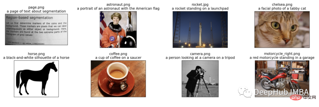
We normalize the image, label each text input, and run the forward propagation of the model to obtain the image and Characteristics of the text.
1 2 3 4 |
|
We normalize the features, calculate the dot product of each pair, and perform cosine similarity calculation
1 2 3 4 5 6 7 8 9 10 11 12 13 14 15 16 17 18 19 20 21 22 23 24 |
|
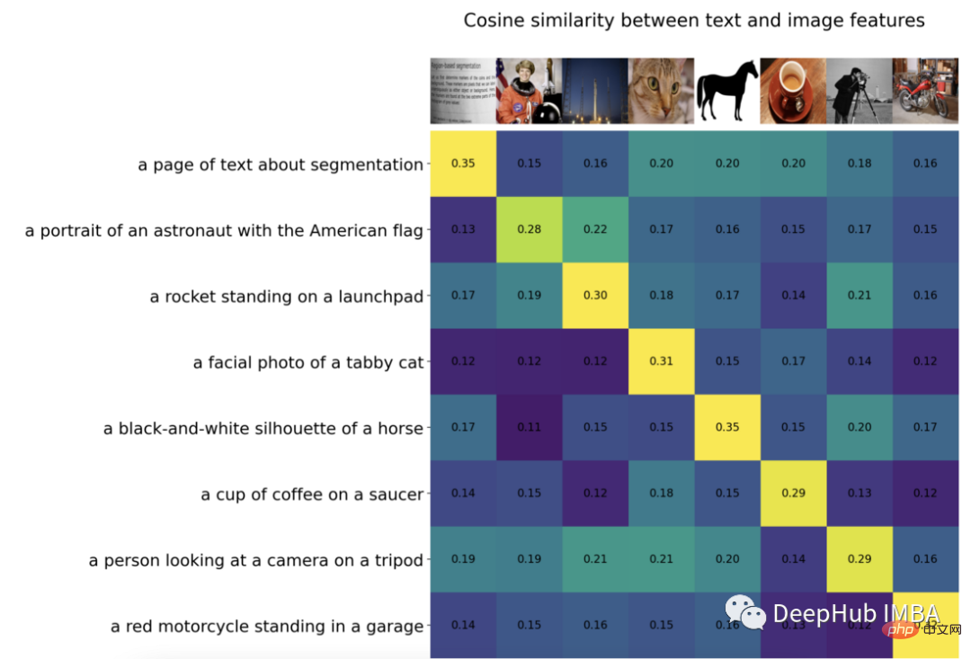
Zero sample image classification
1 2 3 4 5 6 7 8 9 10 11 12 13 14 15 16 17 18 19 20 21 22 23 24 25 26 27 |
|
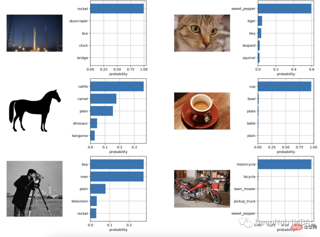
It can be seen that the classification effect is still very good.
The above is the detailed content of Image classification with few-shot learning using PyTorch. For more information, please follow other related articles on the PHP Chinese website!

Hot AI Tools

Undresser.AI Undress
AI-powered app for creating realistic nude photos

AI Clothes Remover
Online AI tool for removing clothes from photos.

Undress AI Tool
Undress images for free

Clothoff.io
AI clothes remover

AI Hentai Generator
Generate AI Hentai for free.

Hot Article

Hot Tools

Notepad++7.3.1
Easy-to-use and free code editor

SublimeText3 Chinese version
Chinese version, very easy to use

Zend Studio 13.0.1
Powerful PHP integrated development environment

Dreamweaver CS6
Visual web development tools

SublimeText3 Mac version
God-level code editing software (SublimeText3)

Hot Topics
 1378
1378
 52
52
 This article will take you to understand SHAP: model explanation for machine learning
Jun 01, 2024 am 10:58 AM
In the fields of machine learning and data science, model interpretability has always been a focus of researchers and practitioners. With the widespread application of complex models such as deep learning and ensemble methods, understanding the model's decision-making process has become particularly important. Explainable AI|XAI helps build trust and confidence in machine learning models by increasing the transparency of the model. Improving model transparency can be achieved through methods such as the widespread use of multiple complex models, as well as the decision-making processes used to explain the models. These methods include feature importance analysis, model prediction interval estimation, local interpretability algorithms, etc. Feature importance analysis can explain the decision-making process of a model by evaluating the degree of influence of the model on the input features. Model prediction interval estimate
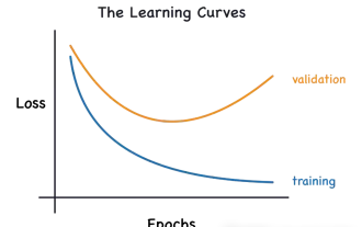 Identify overfitting and underfitting through learning curves
Apr 29, 2024 pm 06:50 PM
This article will introduce how to effectively identify overfitting and underfitting in machine learning models through learning curves. Underfitting and overfitting 1. Overfitting If a model is overtrained on the data so that it learns noise from it, then the model is said to be overfitting. An overfitted model learns every example so perfectly that it will misclassify an unseen/new example. For an overfitted model, we will get a perfect/near-perfect training set score and a terrible validation set/test score. Slightly modified: "Cause of overfitting: Use a complex model to solve a simple problem and extract noise from the data. Because a small data set as a training set may not represent the correct representation of all data." 2. Underfitting Heru
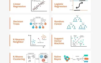 Transparent! An in-depth analysis of the principles of major machine learning models!
Apr 12, 2024 pm 05:55 PM
In layman’s terms, a machine learning model is a mathematical function that maps input data to a predicted output. More specifically, a machine learning model is a mathematical function that adjusts model parameters by learning from training data to minimize the error between the predicted output and the true label. There are many models in machine learning, such as logistic regression models, decision tree models, support vector machine models, etc. Each model has its applicable data types and problem types. At the same time, there are many commonalities between different models, or there is a hidden path for model evolution. Taking the connectionist perceptron as an example, by increasing the number of hidden layers of the perceptron, we can transform it into a deep neural network. If a kernel function is added to the perceptron, it can be converted into an SVM. this one
 The evolution of artificial intelligence in space exploration and human settlement engineering
Apr 29, 2024 pm 03:25 PM
In the 1950s, artificial intelligence (AI) was born. That's when researchers discovered that machines could perform human-like tasks, such as thinking. Later, in the 1960s, the U.S. Department of Defense funded artificial intelligence and established laboratories for further development. Researchers are finding applications for artificial intelligence in many areas, such as space exploration and survival in extreme environments. Space exploration is the study of the universe, which covers the entire universe beyond the earth. Space is classified as an extreme environment because its conditions are different from those on Earth. To survive in space, many factors must be considered and precautions must be taken. Scientists and researchers believe that exploring space and understanding the current state of everything can help understand how the universe works and prepare for potential environmental crises
 Implementing Machine Learning Algorithms in C++: Common Challenges and Solutions
Jun 03, 2024 pm 01:25 PM
Common challenges faced by machine learning algorithms in C++ include memory management, multi-threading, performance optimization, and maintainability. Solutions include using smart pointers, modern threading libraries, SIMD instructions and third-party libraries, as well as following coding style guidelines and using automation tools. Practical cases show how to use the Eigen library to implement linear regression algorithms, effectively manage memory and use high-performance matrix operations.
 Explainable AI: Explaining complex AI/ML models
Jun 03, 2024 pm 10:08 PM
Translator | Reviewed by Li Rui | Chonglou Artificial intelligence (AI) and machine learning (ML) models are becoming increasingly complex today, and the output produced by these models is a black box – unable to be explained to stakeholders. Explainable AI (XAI) aims to solve this problem by enabling stakeholders to understand how these models work, ensuring they understand how these models actually make decisions, and ensuring transparency in AI systems, Trust and accountability to address this issue. This article explores various explainable artificial intelligence (XAI) techniques to illustrate their underlying principles. Several reasons why explainable AI is crucial Trust and transparency: For AI systems to be widely accepted and trusted, users need to understand how decisions are made
 To provide a new scientific and complex question answering benchmark and evaluation system for large models, UNSW, Argonne, University of Chicago and other institutions jointly launched the SciQAG framework
Jul 25, 2024 am 06:42 AM
Editor |ScienceAI Question Answering (QA) data set plays a vital role in promoting natural language processing (NLP) research. High-quality QA data sets can not only be used to fine-tune models, but also effectively evaluate the capabilities of large language models (LLM), especially the ability to understand and reason about scientific knowledge. Although there are currently many scientific QA data sets covering medicine, chemistry, biology and other fields, these data sets still have some shortcomings. First, the data form is relatively simple, most of which are multiple-choice questions. They are easy to evaluate, but limit the model's answer selection range and cannot fully test the model's ability to answer scientific questions. In contrast, open-ended Q&A
 Five schools of machine learning you don't know about
Jun 05, 2024 pm 08:51 PM
Machine learning is an important branch of artificial intelligence that gives computers the ability to learn from data and improve their capabilities without being explicitly programmed. Machine learning has a wide range of applications in various fields, from image recognition and natural language processing to recommendation systems and fraud detection, and it is changing the way we live. There are many different methods and theories in the field of machine learning, among which the five most influential methods are called the "Five Schools of Machine Learning". The five major schools are the symbolic school, the connectionist school, the evolutionary school, the Bayesian school and the analogy school. 1. Symbolism, also known as symbolism, emphasizes the use of symbols for logical reasoning and expression of knowledge. This school of thought believes that learning is a process of reverse deduction, through existing


