

Deep reinforcement learning tackles real-world autonomous driving

arXiv paper "Tackling Real-World Autonomous Driving using Deep Reinforcement Learning", uploaded on July 5, 2022, the author is from Vislab of the University of Parma in Italy and Ambarella (acquisition of Vislab).
In a typical autonomous driving assembly line, the control system represents the two most critical components, in which data retrieved by sensors and data processed by perception algorithms are used to achieve safety Comfortable self-driving behavior. In particular, the planning module predicts the path the self-driving car should follow to perform the correct high-level actions, while the control system performs a series of low-level actions, controlling steering, throttle, and braking.
This work proposes a model-free Deep Reinforcement Learning (DRL) planner to train a neural network to predict acceleration and steering angle, thereby obtaining an autonomous The data driven by the car's positioning and perception algorithms outputs the data driven by the individual modules of the vehicle. In particular, the system that has been fully simulated and trained can drive smoothly and safely in simulated and real (Palma city area) barrier-free environments, proving that the system has good generalization capabilities and can also drive in environments other than training scenarios. In addition, in order to deploy the system on real autonomous vehicles and reduce the gap between simulated performance and real performance, the authors also developed a module represented by a miniature neural network that is able to reproduce the behavior of the real environment during simulation training. Car dynamic behavior.
Over the past few decades, tremendous progress has been made in improving the level of vehicle automation, from simple, rule-based approaches to implementing AI-based intelligent systems. In particular, these systems aim to address the main limitations of rule-based approaches, namely the lack of negotiation and interaction with other road users and the poor understanding of scene dynamics.
Reinforcement Learning (RL) is widely used to solve tasks that use discrete control space outputs, such as Go, Atari games, or chess, as well as autonomous driving in continuous control space. In particular, RL algorithms are widely used in the field of autonomous driving to develop decision-making and maneuver execution systems, such as active lane changes, lane keeping, overtaking maneuvers, intersections and roundabout processing, etc.
This article uses a delayed version of D-A3C, which belongs to the so-called Actor-Critics algorithm family. Specifically composed of two different entities: Actors and Critics. The purpose of the Actor is to select the actions that the agent must perform, while the Critics estimate the state value function, that is, how good the agent's specific state is. In other words, Actors are probability distributions π(a|s; θπ) over actions (where θ are network parameters), and critics are estimated state value functions v(st; θv) = E(Rt|st), where R is Expected returns.
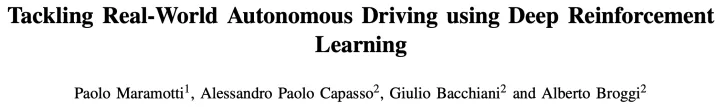
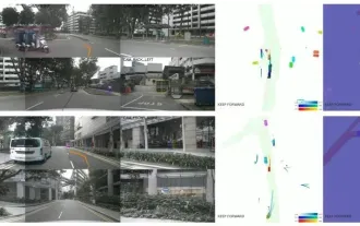
The internally developed high-definition map implements the simulation simulator; an example of the scene is shown in Figure a, which is a partial map area of the real self-driving car test system, while Figure B shows the surrounding view perceived by the agent, Corresponding to an area of 50 × 50 meters, it is divided into four channels: obstacles (Figure c), drivable space (Figure d), the path that the agent should follow (Figure e) and the stop line (Figure f). The high-definition map in the simulator allows retrieving multiple pieces of information about the external environment, such as location or number of lanes, road speed limits, etc.
Focus on achieving a smooth and safe driving style, so the agent is trained in static scenarios, excluding obstacles or other road users, learning to follow routes and respect speed limits .
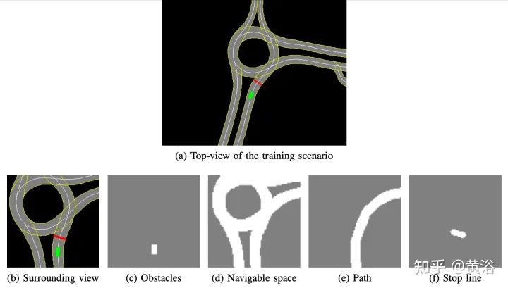
Use the neural network as shown in the figure to train the agent and predict the steering angle and acceleration every 100 milliseconds. It is divided into two sub-modules: the first sub-module can define the steering angle sa, and the second sub-module is used to define the acceleration acc. The inputs to these two submodules are represented by 4 channels (drivable space, path, obstacle and stop line), corresponding to the agent's surrounding view. Each visual input channel contains four 84×84 pixel images to provide the agent with a history of past states. Along with this visual input, the network receives 5 scalar parameters, including the target speed (road speed limit), the agent's current speed, the current speed-target speed ratio, and the final action related to steering angle and acceleration.
In order to ensure exploration, two Gaussian distributions are used to sample the output of the two sub-modules to obtain the relative acceleration (acc=N (μacc, σacc)) and steering Angle (sa=N(μsa,σsa)). The standard deviations σacc and σsa are predicted and modulated by the neural network during the training phase to estimate the uncertainty of the model. In addition, the network uses two different reward functions R-acc-t and R-sa-t, related to acceleration and steering angle respectively, to generate corresponding state value estimates (vacc and vsa).
The neural network was trained on four scenes in the city of Palma. For each scenario, multiple instances are created, and the agents are independent of each other on these instances. Each agent follows the kinematic bicycle model, with a steering angle of [-0.2, 0.2] and an acceleration of [-2.0 m, 2.0 m]. At the beginning of the segment, each agent starts driving at a random speed ([0.0, 8.0]) and follows its intended path, adhering to road speed limits. Road speed limits in this urban area range from 4 ms to 8.3 ms.
Finally, since there are no obstacles in the training scene, the clip can end in one of the following terminal states:
- Achieving the goal: The intelligence reaches the end target location.
- DRIVING OFF THE ROAD: The agent goes beyond its intended path and incorrectly predicts the steering angle.
- Time's Up: The time to complete the fragment has expired; this is primarily due to cautious predictions of acceleration output while driving below the road speed limit.
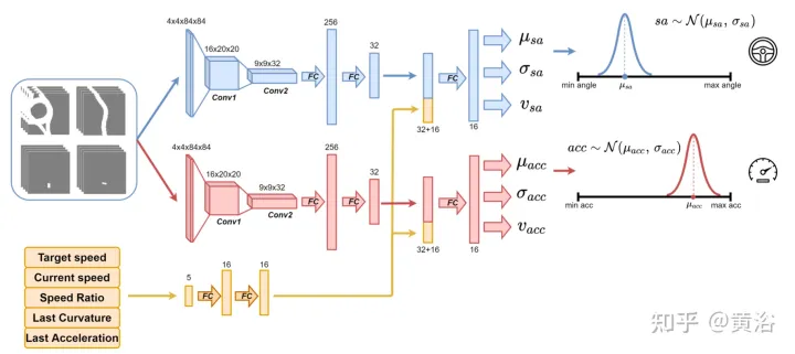
In order to obtain a strategy that can successfully drive a car in simulated and real environments, reward shaping is crucial to achieve the desired behavior. In particular, two different reward functions are defined to evaluate the two actions respectively: R-acc-t and R-sa-t are related to acceleration and steering angle respectively, defined as follows:
where


R-sa-t and R-acc-t both have an element in the formula for Penalize two consecutive actions whose differences in acceleration and steering angle are greater than a certain threshold δacc and δsa respectively. In particular, the difference between two consecutive accelerations is calculated as follows: Δacc=| acc (t) − acc (t− 1) | , while rac_indecision is defined as:

In contrast, the difference between two consecutive predictions of steering angle is calculated as Δsa=| sa(t)−sa(t− 1)|, while rsa_indecision is defined as follows:

Finally, R-acc-t and R-sa-t depend on the terminal state achieved by the agent:
- Goal achieved: The agent reaches the goal position, so the two rewards rterminal is set to 1.0;
- DRIVE OFF ROAD: The agent deviates from its path, mainly due to inaccurate prediction of steering angle. Therefore, assign a negative signal -1.0 to Rsa,t and a negative signal 0.0 to R-acc-t;
- Time is up: the available time to complete the segment expires, mainly due to the agent's acceleration prediction being too Be cautious; therefore, rterminal assumes −1.0 for R-acc-t and 0.0 for R-sa-t.
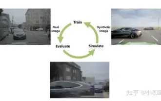
One of the main problems associated with simulators is the difference between simulated and real data, which is caused by the difficulty of truly reproducing real-world conditions within the simulator. To overcome this problem, a synthetic simulator is used to simplify the input to the neural network and reduce the gap between simulated and real data. In fact, the information contained in the 4 channels (obstacles, driving space, path and stop line) as input to the neural network can be easily reproduced by perception and localization algorithms and high-definition maps embedded on real autonomous vehicles.
In addition, another related issue with using simulators has to do with the difference in the two ways in which the simulated agent performs the target action and the self-driving car performs the command. In fact, the target action calculated at time t can ideally take effect immediately at the same precise moment in the simulation. The difference is that this does not happen on a real vehicle, because the reality is that such target actions will be executed with some dynamics, resulting in an execution delay (t δ). Therefore, it is necessary to introduce such response times in simulations in order to train agents on real self-driving cars to handle such delays.
To this end, in order to achieve more realistic behavior, the agent is first trained to add a low-pass filter to the neural network predicted target actions that the agent must perform. As shown in the figure, the blue curve represents the ideal and instantaneous response times occurring in the simulation using the target action (the steering angle of its example). Then, after introducing a low-pass filter, the green curve identifies the simulated agent response time. In contrast, the orange curve shows the behavior of an autonomous vehicle performing the same steering maneuver. However, it can be noticed from the figure that the difference in response time between simulated and real vehicles is still relevant.
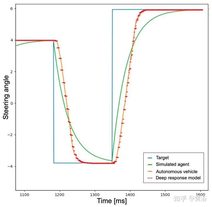
In fact, the acceleration and steering angle points preset by the neural network are not feasible commands, and do not consider some factors, such as the inertia of the system, the delay of the actuator and other non-ideal factors. Therefore, in order to reproduce the dynamics of a real vehicle as realistically as possible, a model consisting of a small neural network consisting of 3 fully connected layers (deep response) was developed. The graph of the depth response behavior is shown as the red dashed line in the figure above, and it can be noticed that it is very similar to the orange curve representing a real self-driving car. Given that the training scene is devoid of obstacles and traffic vehicles, the described problem is more pronounced for steering angle activity, but the same idea has been applied to acceleration output.
Train a deep response model using a dataset collected on a self-driving car, where the inputs correspond to the commands given to the vehicle by the human driver (accelerator pressure and steering wheel turns) and the outputs correspond to the vehicle's throttle, braking and bending , can be measured using GPS, odometer or other technology. In this way, embedding such models in a simulator results in a more scalable system that reproduces the behavior of autonomous vehicles. The depth response module is therefore essential for the correction of steering angle, but even in a less obvious way, it is necessary for acceleration, and this will become clearly visible with the introduction of obstacles.
Two different strategies were tested on real data to verify the impact of the deep response model on the system. Subsequently, verify that the vehicle follows the path correctly and adheres to the speed limits derived from the HD map. Finally, it is proven that pre-training the neural network through Imitation Learning can significantly shorten the total training time.
The strategy is as follows:
- Strategy 1: Do not use the deep response model for training, but use a low-pass filter to simulate the response of the real vehicle to the target action.
- Strategy 2: Ensure more realistic dynamics by introducing a deep response model for training.
Tests performed in simulations produced good results for both strategies. In fact, whether in a trained scene or an untrained map area, the agent can achieve the goal with smooth and safe behavior 100% of the time.
By testing the strategy in real scenarios, different results were obtained. Strategy 1 cannot handle vehicle dynamics and performs predicted actions differently than the agent in the simulation; in this way, Strategy 1 will observe unexpected states of its predictions, leading to noisy behavior on the autonomous vehicle and uncomfortable behaviors.
This behavior also affects the reliability of the system, and in fact, human assistance is sometimes required to avoid the self-driving car from running off the road.
In contrast, in all real-world tests of self-driving cars, Strategy 2 never requires a human to take over, knowing the vehicle dynamics and how the system will evolve to predict actions. The only situations that require human intervention are to avoid other road users; however, these situations are not considered failures because both strategies 1 and 2 are trained in barrier-free scenarios.
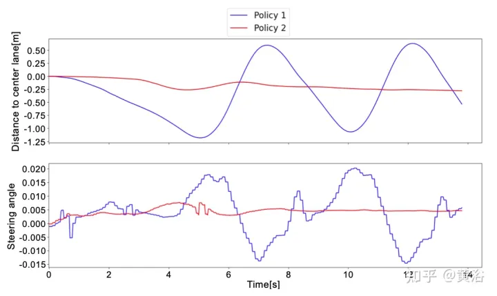
To better understand the difference between Strategy 1 and Strategy 2, here is the steering angle predicted by the neural network and the distance to the center lane within a short window of real-world testing. It can be noticed that the two strategies behave completely different. Strategy 1 (blue curve) is noisy and unsafe compared to strategy 2 (red curve), which proves that the deep response module is important for deployment on truly autonomous vehicles. Strategy is crucial.
To overcome the limitation of RL, which requires millions of segments to reach the optimal solution, pre-training is performed through imitation learning (IL). Furthermore, even though the trend in IL is to train large models, the same small neural network (~1 million parameters) is used, as the idea is to continue training the system using the RL framework to ensure more robustness and generalization capabilities. This way, the usage of hardware resources is not increased, which is crucial considering possible future multi-agent training.
The data set used in the IL training phase is generated by simulated agents that follow a rule-based approach to movement. In particular, for bending, a pure pursuit tracking algorithm is used, where the agent aims to move along a specific waypoint. Instead, use the IDM model to control the longitudinal acceleration of the agent.
To create the dataset, a rule-based agent was moved over four training scenes, saving scalar parameters and four visual inputs every 100 milliseconds. Instead, the output is given by the pure pursuit algorithm and IDM model.
The two horizontal and vertical controls corresponding to the output only represent tuples (μacc, μsa). Therefore, during the IL training phase, the values of the standard deviation (σacc, σsa) are not estimated, nor are the value functions (vacc, vsa) estimated. These features along with the depth response module are learned in the IL RL training phase.
As shown in the figure, it shows the training of the same neural network starting from the pre-training stage (blue curve, IL RL), and compares the results with RL (red curve, pure RL) in four cases. Even though IL RL training requires fewer times than pure RL and the trend is more stable, both methods achieve good success rates (Figure a).
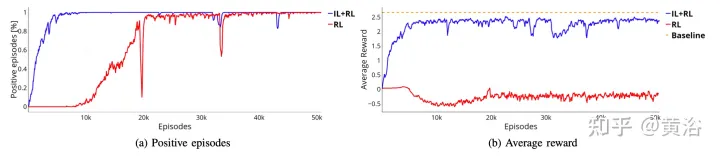
Furthermore, the reward curve shown in Figure b proves that the policy (red curve) obtained using pure RL methods does not even reach an acceptable solution for more training time, while IL RL The policy reaches the optimal solution within a few segments (blue curve in panel b). In this case, the optimal solution is represented by the orange dashed line. This baseline represents the average reward obtained by a simulated agent executing 50,000 segments across 4 scenarios. The simulated agent follows the deterministic rules, which are the same as those used to collect the IL pre-training data set, that is, the pure pursuit rule is used for bending and the IDM rule is used for longitudinal acceleration. The gap between the two approaches may be even more pronounced, training systems to perform more complex maneuvers in which intelligence-body interaction may be required.
The above is the detailed content of Deep reinforcement learning tackles real-world autonomous driving. For more information, please follow other related articles on the PHP Chinese website!

Hot AI Tools

Undresser.AI Undress
AI-powered app for creating realistic nude photos

AI Clothes Remover
Online AI tool for removing clothes from photos.

Undress AI Tool
Undress images for free

Clothoff.io
AI clothes remover

Video Face Swap
Swap faces in any video effortlessly with our completely free AI face swap tool!

Hot Article
Hot Tools

Notepad++7.3.1
Easy-to-use and free code editor

SublimeText3 Chinese version
Chinese version, very easy to use

Zend Studio 13.0.1
Powerful PHP integrated development environment

Dreamweaver CS6
Visual web development tools

SublimeText3 Mac version
God-level code editing software (SublimeText3)
Hot Topics
 1387
1387
 52
52

 Why is Gaussian Splatting so popular in autonomous driving that NeRF is starting to be abandoned?
Jan 17, 2024 pm 02:57 PM
Why is Gaussian Splatting so popular in autonomous driving that NeRF is starting to be abandoned?
Jan 17, 2024 pm 02:57 PM
Written above & the author’s personal understanding Three-dimensional Gaussiansplatting (3DGS) is a transformative technology that has emerged in the fields of explicit radiation fields and computer graphics in recent years. This innovative method is characterized by the use of millions of 3D Gaussians, which is very different from the neural radiation field (NeRF) method, which mainly uses an implicit coordinate-based model to map spatial coordinates to pixel values. With its explicit scene representation and differentiable rendering algorithms, 3DGS not only guarantees real-time rendering capabilities, but also introduces an unprecedented level of control and scene editing. This positions 3DGS as a potential game-changer for next-generation 3D reconstruction and representation. To this end, we provide a systematic overview of the latest developments and concerns in the field of 3DGS for the first time.
 How to solve the long tail problem in autonomous driving scenarios?
Jun 02, 2024 pm 02:44 PM
How to solve the long tail problem in autonomous driving scenarios?
Jun 02, 2024 pm 02:44 PM
Yesterday during the interview, I was asked whether I had done any long-tail related questions, so I thought I would give a brief summary. The long-tail problem of autonomous driving refers to edge cases in autonomous vehicles, that is, possible scenarios with a low probability of occurrence. The perceived long-tail problem is one of the main reasons currently limiting the operational design domain of single-vehicle intelligent autonomous vehicles. The underlying architecture and most technical issues of autonomous driving have been solved, and the remaining 5% of long-tail problems have gradually become the key to restricting the development of autonomous driving. These problems include a variety of fragmented scenarios, extreme situations, and unpredictable human behavior. The "long tail" of edge scenarios in autonomous driving refers to edge cases in autonomous vehicles (AVs). Edge cases are possible scenarios with a low probability of occurrence. these rare events
 Choose camera or lidar? A recent review on achieving robust 3D object detection
Jan 26, 2024 am 11:18 AM
Choose camera or lidar? A recent review on achieving robust 3D object detection
Jan 26, 2024 am 11:18 AM
0.Written in front&& Personal understanding that autonomous driving systems rely on advanced perception, decision-making and control technologies, by using various sensors (such as cameras, lidar, radar, etc.) to perceive the surrounding environment, and using algorithms and models for real-time analysis and decision-making. This enables vehicles to recognize road signs, detect and track other vehicles, predict pedestrian behavior, etc., thereby safely operating and adapting to complex traffic environments. This technology is currently attracting widespread attention and is considered an important development area in the future of transportation. one. But what makes autonomous driving difficult is figuring out how to make the car understand what's going on around it. This requires that the three-dimensional object detection algorithm in the autonomous driving system can accurately perceive and describe objects in the surrounding environment, including their locations,
 Have you really mastered coordinate system conversion? Multi-sensor issues that are inseparable from autonomous driving
Oct 12, 2023 am 11:21 AM
Have you really mastered coordinate system conversion? Multi-sensor issues that are inseparable from autonomous driving
Oct 12, 2023 am 11:21 AM
The first pilot and key article mainly introduces several commonly used coordinate systems in autonomous driving technology, and how to complete the correlation and conversion between them, and finally build a unified environment model. The focus here is to understand the conversion from vehicle to camera rigid body (external parameters), camera to image conversion (internal parameters), and image to pixel unit conversion. The conversion from 3D to 2D will have corresponding distortion, translation, etc. Key points: The vehicle coordinate system and the camera body coordinate system need to be rewritten: the plane coordinate system and the pixel coordinate system. Difficulty: image distortion must be considered. Both de-distortion and distortion addition are compensated on the image plane. 2. Introduction There are four vision systems in total. Coordinate system: pixel plane coordinate system (u, v), image coordinate system (x, y), camera coordinate system () and world coordinate system (). There is a relationship between each coordinate system,
 This article is enough for you to read about autonomous driving and trajectory prediction!
Feb 28, 2024 pm 07:20 PM
This article is enough for you to read about autonomous driving and trajectory prediction!
Feb 28, 2024 pm 07:20 PM
Trajectory prediction plays an important role in autonomous driving. Autonomous driving trajectory prediction refers to predicting the future driving trajectory of the vehicle by analyzing various data during the vehicle's driving process. As the core module of autonomous driving, the quality of trajectory prediction is crucial to downstream planning control. The trajectory prediction task has a rich technology stack and requires familiarity with autonomous driving dynamic/static perception, high-precision maps, lane lines, neural network architecture (CNN&GNN&Transformer) skills, etc. It is very difficult to get started! Many fans hope to get started with trajectory prediction as soon as possible and avoid pitfalls. Today I will take stock of some common problems and introductory learning methods for trajectory prediction! Introductory related knowledge 1. Are the preview papers in order? A: Look at the survey first, p
 Let's talk about end-to-end and next-generation autonomous driving systems, as well as some misunderstandings about end-to-end autonomous driving?
Apr 15, 2024 pm 04:13 PM
Let's talk about end-to-end and next-generation autonomous driving systems, as well as some misunderstandings about end-to-end autonomous driving?
Apr 15, 2024 pm 04:13 PM
In the past month, due to some well-known reasons, I have had very intensive exchanges with various teachers and classmates in the industry. An inevitable topic in the exchange is naturally end-to-end and the popular Tesla FSDV12. I would like to take this opportunity to sort out some of my thoughts and opinions at this moment for your reference and discussion. How to define an end-to-end autonomous driving system, and what problems should be expected to be solved end-to-end? According to the most traditional definition, an end-to-end system refers to a system that inputs raw information from sensors and directly outputs variables of concern to the task. For example, in image recognition, CNN can be called end-to-end compared to the traditional feature extractor + classifier method. In autonomous driving tasks, input data from various sensors (camera/LiDAR
 SIMPL: A simple and efficient multi-agent motion prediction benchmark for autonomous driving
Feb 20, 2024 am 11:48 AM
SIMPL: A simple and efficient multi-agent motion prediction benchmark for autonomous driving
Feb 20, 2024 am 11:48 AM
Original title: SIMPL: ASimpleandEfficientMulti-agentMotionPredictionBaselineforAutonomousDriving Paper link: https://arxiv.org/pdf/2402.02519.pdf Code link: https://github.com/HKUST-Aerial-Robotics/SIMPL Author unit: Hong Kong University of Science and Technology DJI Paper idea: This paper proposes a simple and efficient motion prediction baseline (SIMPL) for autonomous vehicles. Compared with traditional agent-cent
 Reward function design issues in reinforcement learning
Oct 09, 2023 am 11:58 AM
Reward function design issues in reinforcement learning
Oct 09, 2023 am 11:58 AM
Reward function design issues in reinforcement learning Introduction Reinforcement learning is a method that learns optimal strategies through the interaction between an agent and the environment. In reinforcement learning, the design of the reward function is crucial to the learning effect of the agent. This article will explore reward function design issues in reinforcement learning and provide specific code examples. The role of the reward function and the target reward function are an important part of reinforcement learning and are used to evaluate the reward value obtained by the agent in a certain state. Its design helps guide the agent to maximize long-term fatigue by choosing optimal actions.
