
Everyone should have seen "Mission: Impossible 4" directed by Brad Bird and starring Tom Cruise? In a crowded train station, it only takes a blink of an eye to be recognized by the computer and immediately followed by agents; the beautiful woman who meets him is a deadly killer, and the mobile phone beeps with an alarm sound, and the beauty's name and information are already displayed on it. This is the face recognition algorithm that this article wants to introduce, and how to use the public cloud AI platform to train the model.
As one of the earlier mature and widely implemented technologies in the field of artificial intelligence, the purpose of face recognition is to determine the identity of faces in pictures and videos. From facial recognition to unlock and pay on mobile phones, to facial recognition control in the security field, etc., facial recognition technology has a wide range of applications. The face is an innate characteristic of each person. This characteristic is unique and cannot be easily copied, thus providing a necessary prerequisite for identity identification.
Research on face recognition began in the 1960s. With the continuous improvement of computer technology and optical imaging technology, and the resurgence of neural network technology in recent years, especially The great success of convolutional neural networks in image recognition and detection has greatly improved the performance of face recognition systems. In this article, we start with the technical details of face recognition technology and give you a preliminary understanding of the development process of face recognition technology. In the second half of the article, we will use the custom image of the ModelArts platform to show you how to use public Cloud computing resources can quickly train a usable face recognition model.
Whether it is based on traditional image processing and machine learning technology, or using deep learning technology, the process is the same. As shown in Figure 1, face recognition systems include four basic links: face detection, alignment, encoding and matching. Therefore, this part first provides an overview of the face recognition system based on traditional image processing and machine learning algorithms, so that we can see the development context of the entire deep learning algorithm in the field of face recognition.

Face detection process
As mentioned before, face recognition The purpose is to determine the identity of the face in the image, so we first need to detect the face in the image. In fact, this step is ultimately a problem of target detection. The traditional image target detection algorithm mainly consists of three parts, proposal frame generation, feature engineering and classification. The optimization ideas including the famous RCNN series of algorithms are also based on these three parts.
The first is to generate the suggestion frame. The simplest idea for this step is to crop out a bunch of frames to be detected in the picture, and then detect whether there is a target in the frame. If it exists, then the The position of the frame in the original image is the position where the target is detected. Therefore, the greater the coverage of the target in this step, the better the proposed frame generation strategy. Common suggestion box generation strategies include sliding window, Selective Search, Randomized Prim, etc., which generate a large number of candidate boxes, as shown in the figure below.
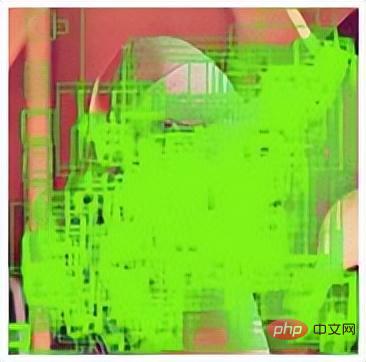
After obtaining a large number of candidate frames, the next most important part of the traditional face detection algorithm is feature engineering. Feature engineering actually uses the expert experience of algorithm engineers to extract various features from faces in different scenes, such as edge features, shape morphology features, texture features, etc. Specific algorithm technologies include LBP, Gabor, Haar, SIFT, etc. Feature extraction algorithm converts a face image represented by a two-dimensional matrix into the representation of various feature vectors.
After obtaining the feature vector, you can classify the feature through traditional machine learning classifiers to determine whether it is a face, such as through adaboost, cascade, SVM, random forest, etc. wait. After classification by a traditional classifier, the face area, feature vector, classification confidence, etc. can be obtained. With this information, we can complete face alignment, feature representation, and face matching recognition.
Take the classic HAAR AdaBoost method as an example among traditional methods. In the feature extraction stage, haar features are first used to extract many simple features from the image. Haar features are shown in the figure below. In order to meet the detection of faces of different sizes, Gaussian pyramid is usually used to extract Haar features from images of different resolutions.

The calculation method of Haar feature is to subtract the black area from the sum of pixels in the white area, so the values obtained are different in the face and non-face areas. Generally, in the specific implementation process, it can be quickly implemented through the integral diagram method. Generally, in the training images normalized to 20*20, the number of available Haar features is about 10,000. Therefore, with this feature scale, machine learning algorithms can be used for classification and identification.
After obtaining the Haar features, you can use Adaboost for classification. The Adaboost algorithm is a combination of multiple weak classification methods to form a new strong classification method. Based on the cascade classifier and the trained feature selection thresholds, the face detection can be completed.
It can be seen from the above method that the traditional machine learning algorithm is a feature-based algorithm, so it requires a large amount of expert experience of algorithm engineers to perform feature engineering and parameter adjustment. The algorithm effect Not very good either. Moreover, it is very difficult for artificial design to be robust to different changing conditions in an unconstrained environment. In the past, image algorithms used traditional image processing methods to extract a large number of features based on real-life scenarios and expert experience, and then performed statistical learning on the extracted features. In this way, the performance of the overall algorithm was very Relying on real-life scenes and expert experience, the effect is not very good for unconstrained scenes with huge categories such as faces and serious imbalance of samples in each category. Therefore, with the great success of deep learning in image processing in recent years, face recognition technology is also based on deep learning, and has achieved very good results.
In the face recognition system of deep learning, the problem is divided into a target detection problem and A classification problem, and the target detection problem is essentially a classification problem and regression problem in deep learning. Therefore, with the successful application of convolutional neural networks in image classification, the effect of the face recognition system has been rapidly and greatly improved. As a result, a large number of visual algorithm companies have been born, and face recognition has been applied to all aspects of social life.
In fact, using neural networks for face recognition is not a new idea. In 1997, researchers proposed a method called based on face detection, eye positioning and face recognition. A neural network approach to probabilistic decision-making. This face recognition PDBNN is divided into a fully connected sub-network for each training subject to reduce the number of hidden units and avoid overfitting. The researchers trained two PBDNNs separately using density and edge features, and then combined their outputs to get the final classification decision. However, due to the serious shortage of computing power and data at the time, the algorithm was relatively simple, so the algorithm did not achieve very good results. With the maturation of backpropagation theory and computing power frameworks only this year, the effectiveness of face recognition algorithms has begun to be greatly improved.
In deep learning, a complete face recognition system also includes the four steps shown in Figure 1. The first step is called the face detection algorithm, which is essentially a target detection algorithm. The second step is called face alignment, which is currently based on geometric alignment of key points and face alignment based on deep learning. The third step is feature representation. In deep learning, through the idea of classification network, some feature layers in the classification network are extracted as the feature representation of the face, and then the standard face image is processed in the same way, and finally through comparison The query method completes the overall face recognition system. The following is a brief overview of the development of face detection and face recognition algorithms.
After the great success of deep learning in image classification, it was quickly used for the problem of face detection. At first, most of the ideas to solve this problem were Based on the scale invariance of the CNN network, the image is scaled at different scales, and then inference is performed and the category and location information are directly predicted. In addition, due to the direct position regression of each point in the feature map, the accuracy of the obtained face frame is relatively low. Therefore, some people have proposed a coarse-to-fine detection strategy based on a multi-stage classifier to detect faces. For example, the main method is Cascade. CNN, DenseBox and MTCNN to name a few.
MTCNN is a multi-task method that puts face area detection and face key point detection together for the first time. Like Cascade CNN, it is also based on the cascade framework, but The overall idea is more clever and reasonable. MTCNN is generally divided into three parts: PNet, RNet and ONet. The network structure is shown in the figure below.
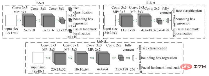
First, the PNet network resizes the input image to different sizes. As input, it directly passes through two layers of convolution and returns the face classification and face detection frame. This part is called rough detection. After cropping the roughly detected face from the original image, perform face detection again on the input R-Net. Finally, the obtained face is finally input into O-Net, and the obtained O-Net output result is the final face detection result. The overall process of MTCNN is relatively simple and can be deployed and implemented quickly. However, MTCNN also has many shortcomings. Including multi-stage task training is time-consuming, and saving a large number of intermediate results requires a large amount of storage space. In addition, since the modified network directly performs bounding box regression on feature points, the effect on small target face detection is not very good. In addition, during the inference process, in order to meet the needs of face detection of different sizes, the network needs to resize the face images to different sizes, which seriously affects the speed of inference.
With the development of the field of target detection, more and more experimental evidence proves that more bottlenecks in target detection lie in low underlying network semantics but relatively high positioning accuracy and high-level network semantics Due to the contradiction of high positioning accuracy but low positioning accuracy, anchor-based strategies and cross-layer fusion strategies have also become popular in target detection networks, such as the famous Faster-rcnn, SSD and yolo series. Therefore, face detection algorithms are increasingly using anchors and multi-channel output to meet the detection effects of faces of different sizes. The most famous algorithm is the SSH network structure.
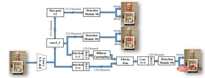
As can be seen from the above figure, the SSH network already has methods for processing the output of different network layers, which can be completed with only one inference. The detection process of faces of different sizes is therefore called Single Stage. The SSH network is also relatively simple, it just performs branch calculations and outputs on different convolutional layers of VGG. In addition, the high-level features are upsampled, and Eltwise Sum is performed with the low-level features to complete the feature fusion of the low-level and high-level features. In addition, the SSH network also designed a detection module and a context module. The context module, as part of the detection module, adopts the inception structure to obtain more contextual information and a larger receptive field.
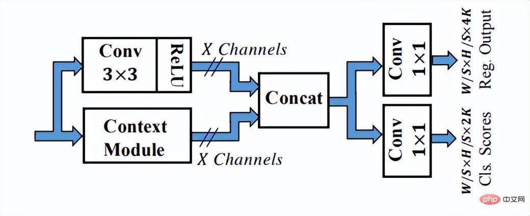
The detection module in SSH

The context module in the detection module in SSH
SSH uses 1×1 convolution to output the final regression and classification branch results, and does not use the fully connected layer, so it can ensure that the input of pictures of different sizes can get the output results, which is also responsive. The trend of fully convolutional design method at that time. Unfortunately, the network does not output landmark points. In addition, the context structure does not use the more popular feature pyramid structure. The backbone of VGG16 is also relatively shallow. With the continuous advancement of face optimization technology, various tricks They are also becoming more mature. Therefore, finally, I would like to introduce to you the Retinaface network, which is widely used in current face detection algorithms.
Retinaface was proposed by Google. It is essentially based on the network structure of RetinaNet and uses feature pyramid technology to achieve the fusion of multi-scale information and plays an important role in detecting small objects. The network structure is shown below.

As can be seen from the above figure, Retinaface’s backbone network is a common convolutional neural network, and then adds the feature pyramid structure and Context Module module , further integrates contextual information, and completes a variety of tasks including classification, detection, landmark point regression, and image self-enhancement.
Because the essence of face detection is a target detection task, the future direction of target detection also applies to the optimization direction of faces. At present, it is still difficult to detect small targets and occluded targets in target detection. In addition, most detection networks are increasingly deployed on the end side. Therefore, network model compression and reconstruction acceleration based on the end side are more challenging for algorithm engineers. Understanding and application of deep learning detection algorithms.
The essence of the face recognition problem is a classification problem, that is, each person is classified and detected as a class, but many problems will arise in the actual application process. First, there are many face categories. If you want to identify everyone in a town, there will be nearly 100,000 categories. In addition, there are very few labeled samples available for each person, and there will be a lot of long-tail data. Based on the above problems, the traditional CNN classification network needs to be modified.
We know that although the deep convolutional network is a black box model, it can characterize the characteristics of pictures or objects through data training. Therefore, the face recognition algorithm can extract a large number of face feature vectors through the convolutional network, and then complete the face recognition process based on similarity judgment and comparison with the base library. Therefore, can the algorithm network generate different features for different faces? Generating similar features for the same face will be the focus of this type of embedding task, that is, how to maximize the inter-class distance and minimize the intra-class distance.
In face recognition, the backbone network can use various convolutional neural networks to complete feature extraction, such as resnet, inception, etc. Classic convolutional neural networks serve as backbone. The key It lies in the design and implementation of the last layer of loss function. Now let’s analyze various loss functions in face recognition algorithms based on deep learning from two ideas.
Idea 1: metric learning, including contrastive loss, triplet loss and sampling method
Idea 2: margin based classification, including softmax with center loss, sphereface, normface, AM-sofrmax(cosface) and arcface.
1. Metric Larning
##(1)Contrastive loss
One of the first applications of metric learning ideas in deep learning is DeepID2. The most important improvement of DeepID2 is that the same network trains verification and classification at the same time (with two supervision signals). Among them, contrastive loss is introduced in the feature layer of verification loss.
Contrastive loss not only considers the distance minimization of the same category, but also considers the distance maximization of different categories. It improves the accuracy of face recognition by making full use of the label information of the training samples. . Therefore, the loss function essentially makes photos of the same person close enough in the feature space, and different people are far enough apart in the feature space until they exceed a certain threshold. (Sounds a bit like triplet loss).

Contrastive loss introduces two signals and trains the network through the two signals. The expression for identifying the signal is as follows:

The expression for verifying the signal is as follows:

Based on this signal, DeepID2 is not trained with one picture as the unit, but with Image Pair as the unit. Each time two pictures are input, it is 1 for the same person. If If they are not the same person, it is -1.
(2)Triplet loss from FaceNet
This article comes from 15 years ago Google's FaceNet is also a watershed work in the field of facial recognition. It proposes a unified solution framework for most face problems, that is, problems such as recognition, verification, and search can all be done in the feature space. What needs to be focused on is how to better map the face to the feature space. .
Based on DeepID2, Google abandoned the classification layer, that is, Classification Loss, and improved Contrastive Loss to Triplet loss, for one purpose only: to learn better features.
Directly post the loss function of Triplet loss. The input is no longer an Image Pair, but three images (Triplet), namely Anchor Face, Negative Face and Positive Face. Anchor and Positive Face are the same person, and Negative Face are different people. Then the loss function of Triplet loss can be expressed as:

The intuitive explanation of this formula is: in the feature space, the distance between Anchor and Positive is smaller than the distance between Anchor and Negative and exceeds a Margin Alpha. The intuitive difference between it and contrastive loss is shown in the figure below.

(3) Problems with Metric learning
The above two The loss function has a very good effect and is in line with people's objective cognition. It has been widely used in actual projects, but this method still has some shortcomings.
2. Various tricks to correct the shortcomings of Metric Learning
(1 ) Finetune
Reference paper: Deep Face Recognition
In the paper "Deep Face Recognition", In order to speed up the training of triplet loss, I first used softmax to train the face recognition model, then removed the top-level classification layer, and then used triplet loss to finetune the feature layer of the model. It also achieved very good results while accelerating training. This method is also the most commonly used method when training triplet loss.
(2) Modification of Triplet loss
Reference paper: In Defense of the Triplet Loss for Person Re-Identification
#The author stated the shortcomings of Triplet loss. For a triplet required for Triplet loss training, anchor(a), positive(p), and negative(n) need to be randomly selected from the training set. Due to the drive of the loss function, it is very likely that a very simple sample combination will be selected, that is, a very similar positive sample and a very similar negative sample. If the network keeps learning on simple samples, it will limit the normalization of the network. ability. Therefore, I modified the triplet loss and added a new trick. A large number of experiments have proven that this improved method works very well.
In the facenet triplet loss training provided by Google, once the B triplets set is selected, the data will be arranged in groups of 3 in order, so there are 3B combinations in total. , but these 3B images actually have as many valid triplets combinations, and using only 3B is wasteful.
In this paper, the author proposed a TriHard loss. The core idea is to add hard example processing on the basis of triplet loss: for each training batch, randomly Select P pedestrians with IDs, and each pedestrian randomly selects K different pictures, that is, a batch contains P×K pictures. Then for each image a in the batch, we can select the most difficult positive sample and the most difficult negative sample to form a triplet with a. First, we define the picture set with the same ID as a as A, and the remaining picture set with different IDs as B. Then the TriHard loss is expressed as:

Among them are the artificially set threshold parameters. TriHard loss will calculate the Euclidean distance between a and each picture in the batch in the feature space, and then select the positive sample p that is farthest (least unlike) from a and the negative sample n that is closest (most similar) to a. Compute triplet loss. where d represents the Euclidean distance. Another way to write the loss function is as follows:
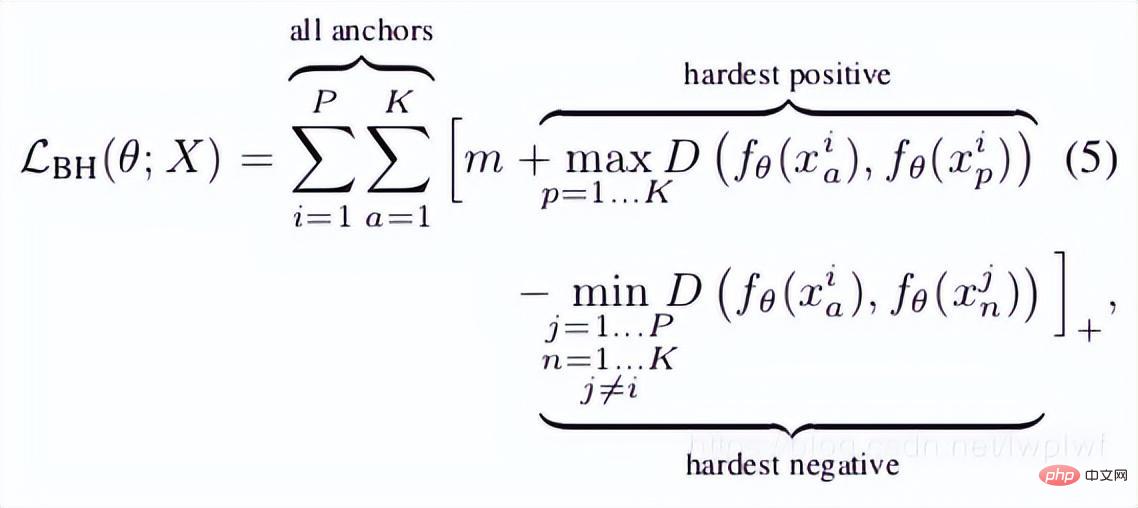
In addition, the author also put forward several experimental points during the round:
This method is better than the traditional triplet loss after taking into account the hard example.
(3) Modifications to loss and sample methods
Reference paper: Deep Metric Learning via Lifted Structured Feature Embedding
This paper first proposes that the existing triplet method cannot fully utilize the advantages of training batches of minibatch SGD training, and creatively uses the vector of pairwise distances were converted into the matrix of pairwise
distance, and then a new structured loss function was designed, which achieved very good results. As shown in the figure below, it is a sampling diagram of the three methods of contrast embedding, triplet embedding and lifted structured embedding.
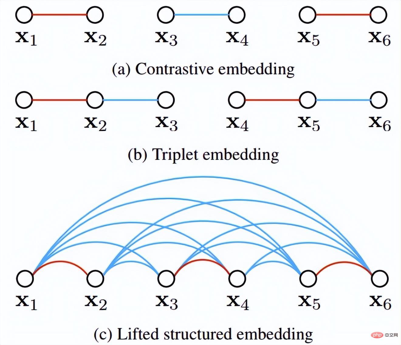
Intuitively, lifted structured embedding involves more classification modes. In order to avoid training difficulties caused by large amounts of data, the author based on this A structured loss function is given. As shown below.

where P is the positive sample set and N is the negative sample set. It can be seen that compared with the above loss function, this loss function starts to consider the problem of a sample set. However, not all negative edges between sample pairs carry useful information. That is to say, the negative edges between randomly sampled sample pairs carry very limited information. Therefore, we need to design a non-random sampling method. .
Through the above structured loss function, we can see that in the final calculation of the loss function, the most similar and least similar hard pairs (that is, the max in the loss function) are considered. Use), which is equivalent to adding difficult
neighbors information to the training mini-batch during the training process. In this way, the training data can search for samples of hard negatives and hard positives with a high probability, and as the training With the continuous progress, the training of hard samples will also achieve the purpose of maximizing the inter-class distance and minimizing the intra-class distance.

As shown in the figure above, this article does not randomly select sample pairs when performing metric learning, but combines multiple types of samples. Train those who are difficult to distinguish between them. In addition, the article also mentioned that the process of seeking max or seeking the single hardest negative will cause the network to converge to a bad local optimum. I guess it may be because of the truncation effect of max, which makes the gradient steeper or has too many gradient discontinuities. The author further improved the loss
function and adopted smooth upper bound, which is shown in the following formula.

(4) Further modifications to the sample method and triplet loss
Reference Paper: Sampling Matters in Deep Embedding Learning
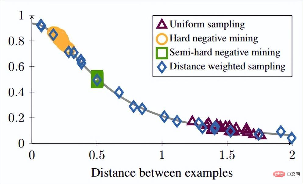
The article points out hard negative Since the anchor distance of the sample is small, if there is noise, then this sampling method will be easily affected by the noise, causing the model to collapse during training. FaceNet once proposed a semi-hard negative mining method. The method it proposed was to make the sampled samples not too hard. However, according to the author's analysis, the sample should be evenly sampled in the sample, so the best sampling state should be in evenly dispersed negative samples, including hard, semi-hard, and easy samples, so The author proposes a new sampling method Distance weighted sampling.
In reality, our team samples all samples in pairs and calculates their distances. Finally, the distribution of point pair distances has the following relationship:

Then based on the given distance, the sampling probability can be obtained through the inverse function of the above function, and the proportion of sampling required for each distance is determined based on this probability. Given an anchor, the probability of sampling a negative example is as follows:

Since the training sample is strongly correlated with the training gradient, the author also plots The relationship between sampling distance, sampling method and data gradient variance is shown in the figure below. As can be seen from the figure, the samples sampled by the hard negative mining method are all in high variance areas. If there is noise in the data set, the sampling will be easily affected by the noise, leading to model collapse. Randomly sampled samples tend to be concentrated in low-variance areas, making the loss very small, but at this time the model is not actually trained well. The sampling range of semi-hard negative mining is very small, which is likely to cause the model to converge very early and the loss to decrease very slowly, but in fact the model has not been trained well at this time; and the method proposed in this article can be achieved in Sample evenly across the entire dataset.
The author is observing the conservative loss and A problem discovered during triplet loss is that the loss function is very smooth when the negative sample is very hard, which means that the gradient will be very small. For training, small gradient means that very hard samples cannot be fully trained, and the network Effective information of hard samples cannot be obtained, so the effect of hard samples will become worse. So if the loss around the hard sample is not so smooth, that is, the derivative often used in deep learning is 1 (like relu), then the hard mode will solve the problem of gradient disappearance. In addition, the loss function must also implement triplet loss to take into account both positive and negative samples, and have the function of margin design, which is to adapt to different data distributions. The loss function is as follows:

We call the distance between the anchor sample and the positive sample the positive sample pair distance; we call the anchor sample and the negative sample The distance between them is the distance between negative pairs. The parameter beta in the formula defines the limit between the distance between the positive pair and the distance between the negative pair. If the distance Dij between the positive pair is greater than beta, the loss will increase; or if the distance Dij between the negative pair is smaller than beta, the loss will increase. A controls the separation interval of samples; when the sample is a positive pair, yij is 1, and when the sample is a negative pair, yij is -1. The figure below shows the loss function curve.

You can see from the picture above why the gradient disappears when it is very hard, because when it is close to the 0 point, it is blue The lines become smoother and smoother, and the gradients become smaller and smaller. In addition, the author has also optimized the settings, added sample bias, category bias and hyper-parameters, further optimized the loss function, and can automatically modify the value according to the training process.
3. Margin Based Classification
Margin based classification is not like metric learning which directly calculates the loss in the feature layer To impose strong intuitive restrictions on the feature, we still treat face recognition as a classification task for training. By modifying the softmax
formula, we indirectly implement margin restrictions on the feature layer, making the final feature obtained by the network more discriminative.
(1) Center loss
## Reference paper: A Discriminative Feature Learning Approach for Deep Face Recognition
This article of ECCV 2016 mainly proposes a new Loss: Center Loss to assist Softmax Loss in face training, in order to compress the same category together and ultimately obtain more discriminative features. . Center loss means: providing a category center for each category and minimizing the distance between each sample in the min-batch and the corresponding category center, so as to achieve the purpose of reducing the intra-class distance. The figure below shows the loss function that minimizes the distance between the sample and the class center.
is the category center corresponding to each sample in each batch. It is the same as the feature dimension and is expressed as a high-dimensional manifold distance using Euclidean distance. Therefore, based on softmax, the loss function of center loss is:

Personally understanding Center loss is like adding clustering to the loss function As the training progresses, the samples are consciously clustered at the center of each batch to further maximize the difference between classes. But I think that for high-dimensional features, Euclidean distance does not reflect the distance of clustering, so such simple clustering cannot achieve better results in high dimensions.
(2) L-Softmax
The purpose of the original Softmax is to multiply vectors Transformed into the relationship between the module of the vector and the angle, that is, on this basis, L-Softmax hopes to add a positive integer variable m, you can see:

The resulting decision boundary can more strictly constrain the above inequalities, making the distance within the class more compact and the distance between classes more differentiated. Therefore, based on the above formula and the formula of softmax, the formula of L-softmax can be obtained as:


Due to cos is a decreasing function, so multiplying by m will make the inner product smaller. Eventually, with training, the distance between the classes themselves will increase. By controlling the size of m, you can see the changes in distance within and between classes. The two-dimensional graph is shown as follows:
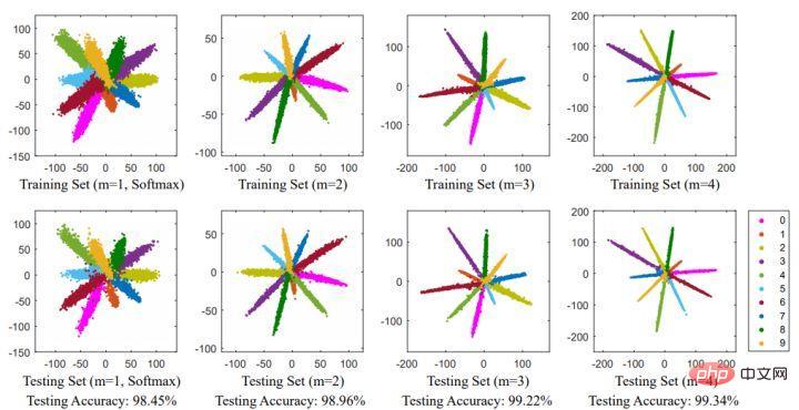
The author in order to ensure that In the process of forward propagation and inference, the angle between the category vectors can satisfy the margin process, and ensure monotonically decreasing, so a new functional form is constructed:

Some people reported that it is difficult to adjust the parameters of L-Softmax, and the parameters of m need to be adjusted repeatedly to achieve better results.
(3)Normface
##Reference paper: NormFace: L2 Hypersphere Embedding for Face Verification
This paper is a very interesting article. The article does a lot of interesting discussions on weights and feature normalization. The article points out that although sphereface is good, it is not beautiful. In the testing phase, sphereface measures the similarity by the cosine value between features, that is, the angle is used as the similarity measure. However, there is also a problem during the training process. The weights are not normalized. While the loss
function decreases during the training process, the module of the weight will become larger and larger, so the optimization direction of the sphereface loss function does not It's not very rigorous. In fact, part of the optimization direction is to increase the length of features. Some bloggers conducted experiments and found that as m increases, the scale of the coordinates also continues to increase, as shown in the figure below.
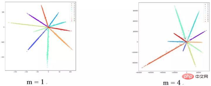
Therefore, the author normalized the features during the optimization process. The corresponding loss function is also as follows:

W and f are both normalized features, and the two dot products are the angle cosine values. The parameter s is introduced because of its mathematical properties, which ensures the rationality of the gradient size. There is a relatively intuitive explanation in the original paper. You can read the original paper, which is not the focus. s can be turned into a learnable parameter or a super parameter. The author of the paper gave many recommended values, which can be found in the paper. In fact, the normalized Euclidean distance and cosine distance in FaceNet are unified.
4. AM-softmax/CosFace
##Reference paper: Additive Margin Softmax for Face Verification
CosFace: Large Margin Cosine Loss for Deep Face Recognition
Looking at the above paper, you will find that there are few One thing is missing, that is, margin, or margin means less, so AM-softmax introduces margin on the basis of normalization. The loss function is as follows:

Intuitively, the -m ratio is smaller, so the loss function value is larger than that in Normface, so there is margin a feeling of. m is a hyperparameter that controls the penalty. The larger m is, the stronger the penalty is. The good thing about this method is that it is easy to reproduce, there are not many parameters adjustment tricks, and the effect is very good.
(1) ArcFace
Compared with AM-softmax, The difference lies in the way Arcface introduces margin. The loss function:

Does it look the same as AM-softmax at first glance? Note that m is inside cosine. The article points out that the boundary between features obtained based on the optimization of the above formula is more superior and has a stronger geometric interpretation.
However, will there be any problems with introducing margin in this way? Think carefully about whether cos(θ m) must be smaller than cos(θ)?
Finally, we use the diagram in the article to explain this problem, and also make a summary of the Margin-based Classification part of this chapter.
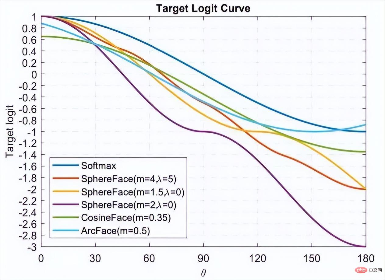
This picture comes from Arcface. The abscissa is θ, which is the angle between the feature and the class center. The ordinate is the value of the numerator index of the loss function. (Regardless of s), the smaller its value, the greater the loss function.
After reading so many classification-based face recognition papers, I believe you also have a feeling that everyone seems to be making a fuss about the loss function, or to be more specific, everyone is discussing How to design the Target logit-θ curve in the figure above.
This curve means how you want to optimize samples that deviate from the target, or in other words, how much punishment you should give based on the degree of deviation from the target. Two points to summarize:
#1. Too strong constraints are not easy to generalize. For example, the loss function of Sphereface can meet the requirement that the maximum distance within a class is smaller than the minimum distance between classes when m=3 or 4. At this time, the loss function value is very large, that is, the target logits is very small. But it does not mean that it can be generalized to samples outside the training set. Imposing too strong constraints will reduce model performance and make training difficult to converge.
2. It is important to choose what kind of samples to optimize. The Arcface article points out that giving too much punishment to samples of θ∈[60°, 90°] may cause the training to not converge. Optimizing samples for θ ∈ [30°, 60°] may improve model accuracy, while over-optimizing samples for θ∈[0°, 30°] will not bring significant improvement. As for samples with larger angles, they deviate too far from the target, and forced optimization is likely to reduce model performance.
This also answers the questions left in the previous section. The curve behind the Arcface in the above picture is rising, which is irrelevant and even beneficial. Because there may be no benefit in optimizing hard samples with large angles. This is the same as the semi-hard strategy for sample selection in FaceNet.
Margin based classification Extended reading1. A discriminative feature learning approach for deep face recognition [14]
Proposed The center loss is weighted and integrated into the original softmax loss. By maintaining a Euclidean space class center, the intra-class distance is reduced and the discriminative power of features is enhanced.
2. Large-margin softmax loss for convolutional neural networks [10]
Sphereface The author's previous article, unnormalized weights, introduced margin in softmax loss. It also involves the training details of Sphereface.
Explanation of face recognition algorithm implementation
The face recognition algorithm we deployed in this article The model mainly consists of two parts:
As shown in the figure below, the overall algorithm implementation process is divided into offline and online parts. Before each identification of different people, first use the training The algorithm generates a standard base database of faces and saves the base database data on modelarts. Then during each inference process, the image input will go through the face detection model and the face recognition model to obtain the face features, and then based on these features, the feature with the highest similarity pair will be searched in the base library to complete the face recognition process.

In the implementation process, we used an algorithm based on Retinaface resnet50 arcface to complete the feature extraction of face images, in which Retinaface is used as the detection model and resnet50 arcface as a feature extraction model.
In the image, there are two scripts for running training, corresponding to face detection training and face recognition training respectively.
run_face_detection_train.sh
The startup command of this script is
<span style="color: rgb(111, 66, 193); margin: 0px; padding: 0px; background: none 0% 0% / auto repeat scroll padding-box border-box rgba(0, 0, 0, 0);">sh</span> run_face_detection_train.sh data_path model_output_path
where model_output_path is the path of the model output, data_path is the input path of the face detection training set, and the input image path structure is as follows:
detection_train_data/train/images/label.txtval/images/label.txttest/images/label.txt
run_face_recognition_train.sh
The startup command of this script is
<span style="color: rgb(111, 66, 193); margin: 0px; padding: 0px; background: none 0% 0% / auto repeat scroll padding-box border-box rgba(0, 0, 0, 0);">sh</span> run_face_recognition_train.sh data_path model_output_path
where model_output_path is the path of the model output, data_path is the input path of the face detection training set. The input image path structure is as follows:
recognition_train_data/cele.idxcele.lstcele.recproperty
run_generate_data_base.sh
The startup command of this script is:
<span style="color: rgb(111, 66, 193); margin: 0px; padding: 0px; background: none 0% 0% / auto repeat scroll padding-box border-box rgba(0, 0, 0, 0);">sh</span> run_generate_data_base.sh data_path detect_model_path recognize_model_path db_output_path
where data_path is the base library input path, detect_model_path is the detection model input path, recognize_model_path is the recognition model input path, and db_output_path is the base Library output path.
run_face_recognition.sh
The startup command of this script is:
<span style="color: rgb(111, 66, 193); margin: 0px; padding: 0px; background: none 0% 0% / auto repeat scroll padding-box border-box rgba(0, 0, 0, 0);">sh</span> run_generate_data_base.sh data_path db_path detect_model_path recognize_model_path
Where data_path is the test image input path, db_path is the base library path, detect_model_path is the input path of the detection model, recognize_model_path is the input path of the recognition model
Huawei Cloud ModelArts has the function of training jobs, which can be used for model training and management of model training parameters and versions. This function is of certain help to developers who are engaged in multi-version iterative development. There are some preset images and algorithms in the training job. Currently, there are preset images for commonly used frameworks (including Caffe, MXNet, Pytorch, TensorFlow) and Huawei's own Ascend chip engine image (Ascend-Powered-Engine).
In this article, based on the custom image feature of ModelArts, we will upload the complete image that we have debugged locally, and use Huawei Cloud's GPU resources to train the model.
We want to use ModelArts on Huawei Cloud to complete a face recognition model based on the data of common celebrities on the website. In this process, since the face recognition network is a network structure designed by engineers themselves, it needs to be uploaded through a custom image. Therefore, the entire face training process is divided into the following nine steps:
Building a local Docker environment
The Docker environment can be built on a local computer, or you can purchase an elastic cloud server on Huawei Cloud to build the Docker environment. Please refer to the official Docker documentation for the entire process:
https://docs.docker.com/engine/install/binaries/#install-static-binaries
Download the basic image from Huawei Cloud
Official website description URL:
https://support.huaweicloud.com/engineers -modelarts/modelarts_23_0085.html#modelarts_23_0085__section19397101102
We need to use the MXNet environment for training. First, we need to download the base image of the corresponding custom image from Huawei Cloud. The download command given by the official website is as follows:

The explanation of this command is found in the specifications of the training job base image.
https://support.huaweicloud.com/engineers-modelarts/modelarts_23_0217.html
According to our script requirements, I used It is the image of cuda9:

The official also provides another method, which is to use docker file. The dockerfile of the base image is also found in the specification of the training job base image. You can refer to the dockerfile:
https://github.com/huaweicloud/ModelArts-Lab/tree/master/docs/custom_image/custom_base
Build a custom image environment according to your own needs
Because I am lazy, I still don’t use Dockerfile to build the image myself. I'm taking another approach!
Because our needs are cuda 9 and some related python dependency packages. Assuming that the official image provides cuda 9, we can follow this tutorial and add it to the training script. a requirement.txt. Simple, efficient and quick solution to your needs! ! ! The following is the tutorial~~~
https://support.huaweicloud.com/modelarts_faq/modelarts_05_0063.html
Upload custom image to SWR
## Official website tutorial:
The page for uploading the image reads , the file must not exceed 2GB after decompression. However, the official basic image provided is 3.11GB. After we add the required pre-trained model, the image is 5 GB, so you cannot use the page to upload, you must use the client. To upload an image, you must first create an organization.

If you find it difficult to understand the product documentation, you can try the pull/push image experience on the SWR page:

The following guides customers on how to push local images to the cloud. The first step is to log in to the warehouse:

The second step is to pull the image. We will replace this with our own custom image.
The third step is to modify the organization and use the organization created according to the product documentation. name. In this step, you need to rename a local image to the image name recognized on the cloud. See the explanation below for details:

The fourth step is to push the image,

When you are proficient in these four steps, you can leave this tutorial and use the client to upload. Log in using the client and upload. Client login can use the temporary docker login command to generate. This page is in "My Image" -> "Client Upload" -> "Generate Temporary Docker Login Instructions":
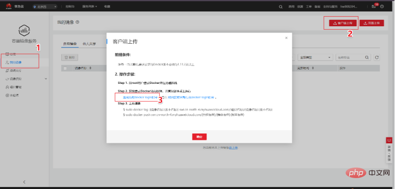
In local docker environment, use the generated temporary docker login command to log in, and use the following command to upload the image:

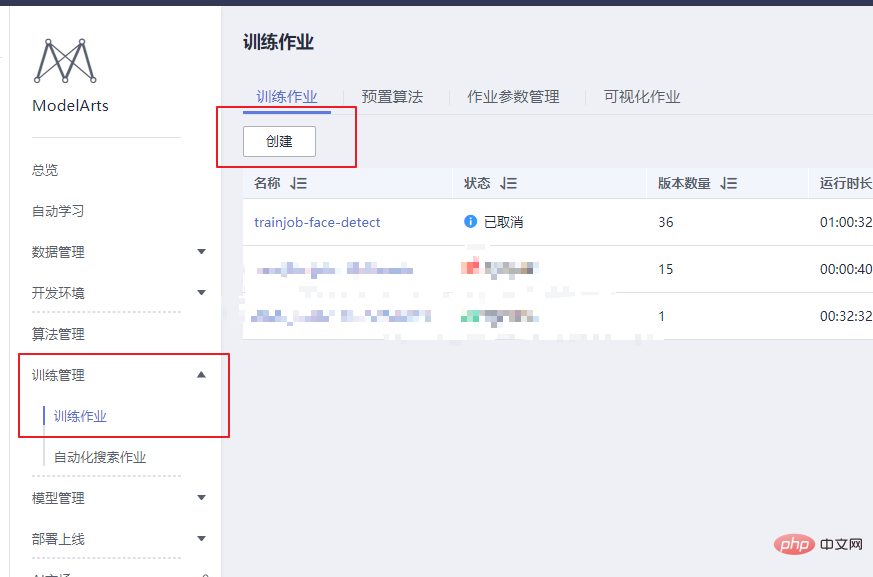
Huawei Cloud ModelArts provides training jobs for users to train models. There are preset images and custom images that can be selected in the training job. The preset images include most of the frameworks on the market. When there are no special requirements, it is also very convenient to use the images of these frameworks for training. This test still uses a custom image.
In a custom image, you not only need to configure your own environment in the image, but if you change the way the training job is started, you also need to modify the training startup script. There is a startup script "run_train.sh" in the /home/work/ path of the official image pulled from the Huawei Cloud ModelArts official website. The customized startup script needs to be modified based on this script. The main thing to pay attention to is
"dls_get_app", which is the command related to downloading from OBS. Other parts are modified according to your own training script.

If you need to upload training results or models to OBS, you need to refer to the "dls_get_app" plus "dls_upload_model" commands. In our training, the uploaded script is as follows:

When debugging the training job, you can currently use the free one-hour V100. One of the better things about the ModelArts training job is that it facilitates our version management. The version will record all parameters passed into the training script through running parameters. You can also use version comparison to compare parameters. Another convenient thing is that it can be modified based on a certain version, which reduces the step of re-entering all parameters and makes debugging more convenient.
After the training is completed in the training job, the model can also be deployed and online in ModelArts.
The current optimization of face recognition algorithms has reached a bottleneck period, but at the technical level, the similarity of facial structure and facial posture , age changes, lighting changes in complex environments, facial ornaments blocking, etc. still face many problems. Therefore, solving various problems in face recognition based on the integration of multiple algorithm technologies still has a huge market in security and the Internet. . In addition, with the gradual improvement of face payment, face recognition systems are also used in banks, shopping malls, etc. Therefore, the security issues and anti-attack issues of face recognition are also urgent issues to be solved, such as liveness detection, 3D facial recognition, etc. wait.
Finally, face recognition is a relatively mature project in deep learning. Its development is also closely related to the technical development of deep learning itself. Currently, in many optimizations, the biggest shortcoming of deep learning is that there is no corresponding mathematical theory. The performance improved by support and optimization is also very limited, so the research on the deep learning algorithm itself is also the focus of the future.
The above is the detailed content of Understand the development trend of face recognition algorithm technology in one article. For more information, please follow other related articles on the PHP Chinese website!
 Detailed explanation of linux dd command
 Unable to start your computer properly
 How to open TIF format in windows
 wap browser
 How to open url file
 Win11 My Computer Added to Desktop Tutorial
 How to use btbook magnetic search
 How to solve the problem that wlan does not have a valid ip configuration
 Main contents of database conceptual design


