Using Pytorch to implement contrastive learning SimCLR for self-supervised pre-training

SimCLR (Simple Framework for Contrastive Learning of Representations) is a self-supervised technology for learning image representations. Unlike traditional supervised learning methods, SimCLR does not rely on labeled data to learn useful representations. It utilizes a contrastive learning framework to learn a set of useful features that can capture high-level semantic information from unlabeled images.

SimCLR has been proven to outperform state-of-the-art unsupervised learning methods on various image classification benchmarks. And the representations it learns can be easily transferred to downstream tasks such as object detection, semantic segmentation and few-shot learning with minimal fine-tuning on smaller labeled datasets.

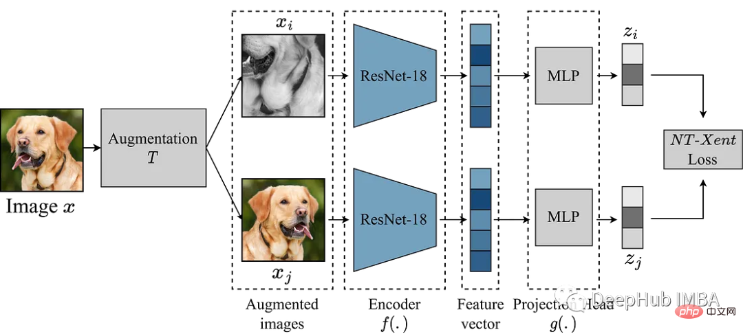
#The main idea of ​​SimCLR is to learn a good representation of the image by comparing it with other enhanced versions of the same image through the enhancement module T. This is done by mapping the image through an encoder network f(.) and then projecting it. head g(.) maps the learned features into a low-dimensional space. A contrastive loss is then calculated between representations of two enhanced versions of the same image to encourage similar representations of the same image and different representations of different images.

In this article we will delve into the SimCLR framework and explore the key components of the algorithm, including data augmentation, contrastive loss functions, and the head architecture of the encoder and projection.

We use the garbage classification data set from Kaggle to conduct experiments

Enhancement module

The most important thing in SimCLR is the enhancement module for converting images. The authors of the SimCLR paper suggest that powerful data augmentation is useful for unsupervised learning. Therefore, we will follow the approach recommended in the paper.

• Random cropping for resizing
• Random horizontal flipping with 50% probability
• Random color distortion (80% probability of color dithering, 20% probability of color drop) )
• 50% probability is random Gaussian blur

def get_complete_transform(output_shape, kernel_size, s=1.0):
 """
Color distortion transform

Args:
s: Strength parameter

Returns:
A color distortion transform
"""
 rnd_crop = RandomResizedCrop(output_shape)
 rnd_flip = RandomHorizontalFlip(p=0.5)

 color_jitter = ColorJitter(0.8*s, 0.8*s, 0.8*s, 0.2*s)
 rnd_color_jitter = RandomApply([color_jitter], p=0.8)

 rnd_gray = RandomGrayscale(p=0.2)
 gaussian_blur = GaussianBlur(kernel_size=kernel_size)
 rnd_gaussian_blur = RandomApply([gaussian_blur], p=0.5)
 to_tensor = ToTensor()
 image_transform = Compose([
 to_tensor,
 rnd_crop,
 rnd_flip,
 rnd_color_jitter,
 rnd_gray,
 rnd_gaussian_blur,
])
 return image_transform

 class ContrastiveLearningViewGenerator(object):
 """
Take 2 random crops of 1 image as the query and key.
"""
 def __init__(self, base_transform, n_views=2):
 self.base_transform = base_transform
 self.n_views = n_views

 def __call__(self, x):
 views = [self.base_transform(x) for i in range(self.n_views)]
 return views

The next step is to define a PyTorch Dataset.

class CustomDataset(Dataset):
 def __init__(self, list_images, transform=None):
 """
Args:
list_images (list): List of all the images
transform (callable, optional): Optional transform to be applied on a sample.
"""
 self.list_images = list_images
 self.transform = transform

 def __len__(self):
 return len(self.list_images)

 def __getitem__(self, idx):
 if torch.is_tensor(idx):
 idx = idx.tolist()

 img_name = self.list_images[idx]
 image = io.imread(img_name)
 if self.transform:
 image = self.transform(image)

 return image

As an example, we use the smaller model ResNet18 as the backbone, so its input is a 224x224 image. We set some parameters as required and generate dataloader

out_shape = [224, 224]
 kernel_size = [21, 21] # 10% of out_shape

 # Custom transform
 base_transforms = get_complete_transform(output_shape=out_shape, kernel_size=kernel_size, s=1.0)
 custom_transform = ContrastiveLearningViewGenerator(base_transform=base_transforms)

 garbage_ds = CustomDataset(
 list_images=glob.glob("/kaggle/input/garbage-classification/garbage_classification/*/*.jpg"),
 transform=custom_transform
 )

 BATCH_SZ = 128

 # Build DataLoader
 train_dl = torch.utils.data.DataLoader(
 garbage_ds,
 batch_size=BATCH_SZ,
 shuffle=True,
 drop_last=True,
 pin_memory=True)

SimCLR

We have prepared the data and started to reproduce the model. The above enhancement module provides two enhanced views of the image, which are forward passed through the encoder to obtain the corresponding representation. The goal of SimCLR is to maximize the similarity between these different learned representations by encouraging the model to learn a general representation of an object from two different augmented views.

The choice of encoder network is not restricted and can be of any architecture. As mentioned above, for simple demonstration, we use ResNet18. The representations learned by the encoder model determine the similarity coefficients, and to improve the quality of these representations, SimCLR uses a projection head to project the encoding vectors into a richer latent space. Here we project the 512-dimensional features of ResNet18 into a 256-dimensional space. It looks very complicated, but in fact it is just adding an mlp with relu.

class Identity(nn.Module):
 def __init__(self):
 super(Identity, self).__init__()
 def forward(self, x):
 return x

 class SimCLR(nn.Module):
 def __init__(self, linear_eval=False):
 super().__init__()
 self.linear_eval = linear_eval
 resnet18 = models.resnet18(pretrained=False)
 resnet18.fc = Identity()
 self.encoder = resnet18
 self.projection = nn.Sequential(
 nn.Linear(512, 512),
 nn.ReLU(),
 nn.Linear(512, 256)
)
 def forward(self, x):
 if not self.linear_eval:
 x = torch.cat(x, dim=0)
 encoding = self.encoder(x)
 projection = self.projection(encoding)
 return projection

Contrast loss

The contrast loss function, also known as the normalized temperature scaled cross-entropy loss (NT-Xent), is a key component of SimCLR , which encourages the model to learn similar representations for the same image and different representations for different images.

NT-Xent loss is computed using a pair of augmented views of an image passed through the encoder network to obtain their corresponding representations. The goal of contrastive loss is to encourage representations of two augmented views of the same image to be similar while forcing representations of different images to be dissimilar.

NT-Xent applies a softmax function to enhance pairwise similarity of view representations. The softmax function is applied to all pairs of representations within the mini-batch to obtain a similarity probability distribution for each image. The temperature parameter is used to scale the pairwise similarities before applying the softmax function, which helps to obtain better gradients during optimization.

After obtaining the probability distribution of similarities, the NT-Xent loss is calculated by maximizing the log-likelihood of matching representations of the same image and minimizing the log-likelihood of mismatching representations of different images.

LABELS = torch.cat([torch.arange(BATCH_SZ) for i in range(2)], dim=0)
 LABELS = (LABELS.unsqueeze(0) == LABELS.unsqueeze(1)).float() #one-hot representations
 LABELS = LABELS.to(DEVICE)

 def ntxent_loss(features, temp):
 """
NT-Xent Loss.

Args:
z1: The learned representations from first branch of projection head
z2: The learned representations from second branch of projection head
Returns:
Loss
"""
 similarity_matrix = torch.matmul(features, features.T)
 mask = torch.eye(LABELS.shape[0], dtype=torch.bool).to(DEVICE)
 labels = LABELS[~mask].view(LABELS.shape[0], -1)
 similarity_matrix = similarity_matrix[~mask].view(similarity_matrix.shape[0], -1)

 positives = similarity_matrix[labels.bool()].view(labels.shape[0], -1)

 negatives = similarity_matrix[~labels.bool()].view(similarity_matrix.shape[0], -1)

 logits = torch.cat([positives, negatives], dim=1)
 labels = torch.zeros(logits.shape[0], dtype=torch.long).to(DEVICE)

 logits = logits / temp
 return logits, labels

All preparations are completed, let’s train SimCLR and see the effect!

simclr_model = SimCLR().to(DEVICE)
 criterion = nn.CrossEntropyLoss().to(DEVICE)
 optimizer = torch.optim.Adam(simclr_model.parameters())

 epochs = 10
 with tqdm(total=epochs) as pbar:
 for epoch in range(epochs):
 t0 = time.time()
 running_loss = 0.0
 for i, views in enumerate(train_dl):
 projections = simclr_model([view.to(DEVICE) for view in views])
 logits, labels = ntxent_loss(projections, temp=2)
 loss = criterion(logits, labels)
 optimizer.zero_grad()
 loss.backward()
 optimizer.step()

 # print stats
 running_loss += loss.item()
 if i%10 == 9: # print every 10 mini-batches
 print(f"Epoch: {epoch+1} Batch: {i+1} Loss: {(running_loss/100):.4f}")
 running_loss = 0.0
 pbar.update(1)
 print(f"Time taken: {((time.time()-t0)/60):.3f} mins")

The above code is trained for 10 rounds. Assuming that we have completed the pre-training process, we can use the pre-trained encoder for the downstream tasks we want. This can be done with the code below.

from torchvision.transforms import Resize, CenterCrop
 resize = Resize(255)
 ccrop = CenterCrop(224)
 ttensor = ToTensor()

 custom_transform = Compose([
 resize,
 ccrop,
 ttensor,
 ])

 garbage_ds = ImageFolder(
 root="/kaggle/input/garbage-classification/garbage_classification/",
 transform=custom_transform
 )

 classes = len(garbage_ds.classes)

 BATCH_SZ = 128

 train_dl = torch.utils.data.DataLoader(
 garbage_ds,
 batch_size=BATCH_SZ,
 shuffle=True,
 drop_last=True,
 pin_memory=True,
 )

 class Identity(nn.Module):
 def __init__(self):
 super(Identity, self).__init__()
 def forward(self, x):
 return x

 class LinearEvaluation(nn.Module):
 def __init__(self, model, classes):
 super().__init__()
 simclr = model
 simclr.linear_eval=True
 simclr.projection = Identity()
 self.simclr = simclr
 for param in self.simclr.parameters():
 param.requires_grad = False
 self.linear = nn.Linear(512, classes)
 def forward(self, x):
 encoding = self.simclr(x)
 pred = self.linear(encoding)
 return pred

 eval_model = LinearEvaluation(simclr_model, classes).to(DEVICE)
 criterion = nn.CrossEntropyLoss().to(DEVICE)
 optimizer = torch.optim.Adam(eval_model.parameters())

 preds, labels = [], []
 correct, total = 0, 0

 with torch.no_grad():
 t0 = time.time()
 for img, gt in tqdm(train_dl):
 image = img.to(DEVICE)
 label = gt.to(DEVICE)
 pred = eval_model(image)
 _, pred = torch.max(pred.data, 1)
 total += label.size(0)
 correct += (pred == label).float().sum().item()

 print(f"Time taken: {((time.time()-t0)/60):.3f} mins")

 print(
 "Accuracy of the network on the {} Train images: {} %".format(
 total, 100 * correct / total
)
)

The most important part of the above code is to read the simclr model just trained, then freeze all the weights, and then create a classification head self.linear to perform downstream classification tasks

Summary

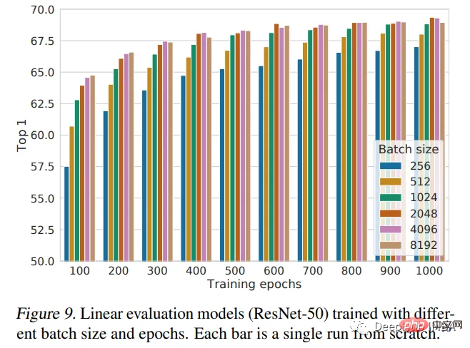
This article introduces the SimCLR framework and uses it to pre-train ResNet18 with randomly initialized weights. Pretraining is a powerful technique used in deep learning to train models on large datasets and learn useful features that can be transferred to other tasks. The SimCLR paper believes that the larger the batch size, the better the performance. Our implementation only uses a batch size of 128 and trains for only 10 epochs. So this is not the best performance of the model. If performance comparison is required, further training is required.

The following figure is the performance conclusion given by the author of the paper:

The above is the detailed content of Using Pytorch to implement contrastive learning SimCLR for self-supervised pre-training. For more information, please follow other related articles on the PHP Chinese website!