
 Technology peripherals
AI
PyTorch parallel training DistributedDataParallel complete code example
Technology peripherals
AI
PyTorch parallel training DistributedDataParallel complete code example
PyTorch parallel training DistributedDataParallel complete code example

The problem of training large deep neural networks (DNN) using large datasets is a major challenge in the field of deep learning. As DNN and dataset sizes increase, so do the computational and memory requirements for training these models. This makes it difficult or even impossible to train these models on a single machine with limited computing resources. Some of the major challenges of training large DNNs using large datasets include:
- Long training time: The training process can take weeks or even months to complete, depending on the complexity of the model and the size of the dataset .
- Memory limitations: Large DNNs may require large amounts of memory to store all model parameters, gradients, and intermediate activations during training. This can cause out-of-memory errors and limit the size of the model that can be trained on a single machine.
To address these challenges, various techniques have been developed to scale up the training of large DNNs with large datasets, including model parallelism, data parallelism, and hybrid parallelism, as well as hardware, software, and Algorithm optimization.
In this article we will demonstrate data parallelism and model parallelism using PyTorch.

What we call parallelism generally refers to training deep neural networks (dnn) on multiple GPUs or multiple machines to achieve Less training time. The basic idea behind data parallelism is to split the training data into smaller chunks and let each GPU or machine process a separate chunk of data. The results for each node are then combined and used to update model parameters. In data parallelism, the model architecture is the same on each node, but the model parameters are partitioned between nodes. Each node trains its own local model using allocated chunks of data, and at the end of each training iteration, the model parameters are synchronized across all nodes. This process is repeated until the model converges to a satisfactory result.
Below we use the ResNet50 and CIFAR10 data sets for a complete code example:
In data parallelism, the model architecture remains the same on each node, but the model parameters are between nodes. Partitioning is done, and each node trains its own local model using the allocated data chunks.
PyTorch's DistributedDataParallel library can efficiently communicate and synchronize gradients and model parameters across nodes to achieve distributed training. This article provides an example of how to implement data parallelism with PyTorch using the ResNet50 and CIFAR10 datasets, where the code is run on multiple GPUs or machines, with each machine processing a subset of the training data. The training process is parallelized using PyTorch's DistributedDataParallel library.
Import the necessary libraries
import os
 from datetime import datetime
 from time import time
 import argparse
 import torchvision
 import torchvision.transforms as transforms
 import torch
 import torch.nn as nn
 import torch.distributed as dist
 from torch.nn.parallel import DistributedDataParallel
Next, we will check the GPU.
import subprocess
 result = subprocess.run(['nvidia-smi'], stdout=subprocess.PIPE)
 print(result.stdout.decode())
Because we need to run on multiple servers, it is not practical to execute them one by one manually, so a scheduler is needed. Here we use a SLURM file to run the code (slurmFree and open source job scheduler for Linux and Unix-like kernels),
def main():

 # get distributed configuration from Slurm environment

 parser = argparse.ArgumentParser()
 parser.add_argument('-b', '--batch-size', default=128, type =int,
 help='batch size. it will be divided in mini-batch for each worker')
 parser.add_argument('-e','--epochs', default=2, type=int, metavar='N',
 help='number of total epochs to run')
 parser.add_argument('-c','--checkpoint', default=None, type=str,
 help='path to checkpoint to load')
 args = parser.parse_args()

 rank = int(os.environ['SLURM_PROCID'])
 local_rank = int(os.environ['SLURM_LOCALID'])
 size = int(os.environ['SLURM_NTASKS'])
 master_addr = os.environ["SLURM_SRUN_COMM_HOST"]
 port = "29500"
 node_id = os.environ['SLURM_NODEID']
 ddp_arg = [rank, local_rank, size, master_addr, port, node_id]
train(args, ddp_arg)Then, we use the DistributedDataParallel library to perform distributed training.
def train(args, ddp_arg):

 rank, local_rank, size, MASTER_ADDR, port, NODE_ID = ddp_arg

 # display info
 if rank == 0:
 #print(">>> Training on ", len(hostnames), " nodes and ", size, " processes, master node is ", MASTER_ADDR)
 print(">>> Training on ", size, " GPUs, master node is ", MASTER_ADDR)
 #print("- Process {} corresponds to GPU {} of node {}".format(rank, local_rank, NODE_ID))

 print("- Process {} corresponds to GPU {} of node {}".format(rank, local_rank, NODE_ID))


 # configure distribution method: define address and port of the master node and initialise communication backend (NCCL)
 #dist.init_process_group(backend='nccl', init_method='env://', world_size=size, rank=rank)
 dist.init_process_group(
 backend='nccl',
 init_method='tcp://{}:{}'.format(MASTER_ADDR, port),
 world_size=size,
 rank=rank
)

 # distribute model
 torch.cuda.set_device(local_rank)
 gpu = torch.device("cuda")
 #model = ResNet18(classes=10).to(gpu)
 model = torchvision.models.resnet50(pretrained=False).to(gpu)
 ddp_model = DistributedDataParallel(model, device_ids=[local_rank])
 if args.checkpoint is not None:
 map_location = {'cuda:%d' % 0: 'cuda:%d' % local_rank}
 ddp_model.load_state_dict(torch.load(args.checkpoint, map_location=map_location))

 # distribute batch size (mini-batch)
 batch_size = args.batch_size
 batch_size_per_gpu = batch_size // size

 # define loss function (criterion) and optimizer
 criterion = nn.CrossEntropyLoss()
 optimizer = torch.optim.SGD(ddp_model.parameters(), 1e-4)


 transform_train = transforms.Compose([
 transforms.RandomCrop(32, padding=4),
 transforms.RandomHorizontalFlip(),
 transforms.ToTensor(),
 transforms.Normalize((0.4914, 0.4822, 0.4465), (0.2023, 0.1994, 0.2010)),
])

 # load data with distributed sampler
 #train_dataset = torchvision.datasets.CIFAR10(root='./data',
 # train=True,
 # transform=transform_train,
 # download=False)

 # load data with distributed sampler
 train_dataset = torchvision.datasets.CIFAR10(root='./data',
train=True,
transform=transform_train,
download=False)

 train_sampler = torch.utils.data.distributed.DistributedSampler(train_dataset,
 num_replicas=size,
 rank=rank)

 train_loader = torch.utils.data.DataLoader(dataset=train_dataset,
batch_size=batch_size_per_gpu,
shuffle=False,
num_workers=0,
pin_memory=True,
sampler=train_sampler)

 # training (timers and display handled by process 0)
 if rank == 0: start = datetime.now()
 total_step = len(train_loader)

 for epoch in range(args.epochs):
 if rank == 0: start_dataload = time()

 for i, (images, labels) in enumerate(train_loader):

 # distribution of images and labels to all GPUs
 images = images.to(gpu, non_blocking=True)
 labels = labels.to(gpu, non_blocking=True)

 if rank == 0: stop_dataload = time()

 if rank == 0: start_training = time()

 # forward pass
 outputs = ddp_model(images)
 loss = criterion(outputs, labels)

 # backward and optimize
 optimizer.zero_grad()
 loss.backward()
 optimizer.step()

 if rank == 0: stop_training = time()
 if (i + 1) % 10 == 0 and rank == 0:
 print('Epoch [{}/{}], Step [{}/{}], Loss: {:.4f}, Time data load: {:.3f}ms, Time training: {:.3f}ms'.format(epoch + 1, args.epochs,
 i + 1, total_step, loss.item(), (stop_dataload - start_dataload)*1000,
(stop_training - start_training)*1000))
 if rank == 0: start_dataload = time()

 #Save checkpoint at every end of epoch
 if rank == 0:
 torch.save(ddp_model.state_dict(), './checkpoint/{}GPU_{}epoch.checkpoint'.format(size, epoch+1))

 if rank == 0:
 print(">>> Training complete in: " + str(datetime.now() - start))


 if __name__ == '__main__':

main()The code splits the data and model across multiple GPUs and updates the model in a distributed manner. Here are some explanations of the code:
train(args, ddp_arg) has two parameters, args and ddp_arg, where args is the command line parameter passed to the script, and ddp_arg contains distributed training related parameters.
rank, local_rank, size, MASTER_ADDR, port, NODE_ID = ddp_arg: Unpack the distributed training related parameters in ddp_arg.
If rank is 0, print the number of GPUs currently used and the master node IP address information.
dist.init_process_group(backend='nccl', init_method='tcp://{}:{}'.format(MASTER_ADDR, port), world_size=size, rank=rank): Use NCCL backend Initialize the distributed process group.
torch.cuda.set_device(local_rank): Select the specified GPU for this process.
model = torchvision.models. ResNet50 (pretrained=False).to(gpu): Load the ResNet50 model from the torchvision model and move it to the specified gpu.
ddp_model = DistributedDataParallel(model, device_ids=[local_rank]): Wrap the model in the DistributedDataParallel module, which means that we can perform distributed training
Load CIFAR-10 data Collect and apply data augmentation transformations.
train_sampler=torch.utils.data.distributed.DistributedSampler(train_dataset,num_replicas=size,rank=rank): Create a DistributedSampler object to split the data set onto multiple GPUs.
train_loader =torch.utils.data.DataLoader(dataset=train_dataset,batch_size=batch_size_per_gpu,shuffle=False,num_workers=0,pin_memory=True,sampler=train_sampler): Create a DataLoader object and the data will be loaded in batches In the model, this is consistent with our usual training steps, except that a distributed data sampling DistributedSampler is added.
Train the model for the specified number of epochs, and use optimizer.step() to update the weights in a distributed manner.
rank0 saves a checkpoint at the end of each round.
rank0 shows loss and training time every 10 batches.
At the end of training, the total time spent on printing the training model is also in rank0.
Code test
Training was conducted using 1 node with 1/2/3/4 GPUs, 2 nodes with 6/8 GPUs, and each node with 3/4 GPUs The test of Resnet50 on Cifar10 is shown in the figure below. The batch size of each test remains the same. The time taken to complete each test was recorded in seconds. As the number of GPUs used increases, the time required to complete the test decreases. When using 8 GPUs, it took 320 seconds to complete, which is the fastest time recorded. This is for sure, but we can see that the training speed does not increase linearly with the increase in the number of GPUs. This may be because Resnet50 is a relatively small model and does not require parallel training.

Using data parallelism on multiple GPUs can significantly reduce the time required to train a deep neural network (DNN) on a given dataset . As the number of GPUs increases, the time required to complete the training process decreases, indicating that DNNs can be trained more efficiently in parallel.
This approach is particularly useful when dealing with large data sets or complex DNN architectures. By leveraging multiple GPUs, the training process can be accelerated, allowing for faster model iteration and experimentation. However, it should be noted that the performance improvements achieved through Data Parallelism may be limited by factors such as communication overhead and GPU memory limitations, and require careful tuning to obtain the best results.
The above is the detailed content of PyTorch parallel training DistributedDataParallel complete code example. For more information, please follow other related articles on the PHP Chinese website!

Hot AI Tools

Undresser.AI Undress
AI-powered app for creating realistic nude photos

AI Clothes Remover
Online AI tool for removing clothes from photos.

Undress AI Tool
Undress images for free

Clothoff.io
AI clothes remover

AI Hentai Generator
Generate AI Hentai for free.

Hot Article
Hot Tools

Notepad++7.3.1
Easy-to-use and free code editor

SublimeText3 Chinese version
Chinese version, very easy to use

Zend Studio 13.0.1
Powerful PHP integrated development environment

Dreamweaver CS6
Visual web development tools

SublimeText3 Mac version
God-level code editing software (SublimeText3)
Hot Topics
 1378
1378
 52
52

 Methods and steps for using BERT for sentiment analysis in Python
Jan 22, 2024 pm 04:24 PM
Methods and steps for using BERT for sentiment analysis in Python
Jan 22, 2024 pm 04:24 PM
BERT is a pre-trained deep learning language model proposed by Google in 2018. The full name is BidirectionalEncoderRepresentationsfromTransformers, which is based on the Transformer architecture and has the characteristics of bidirectional encoding. Compared with traditional one-way coding models, BERT can consider contextual information at the same time when processing text, so it performs well in natural language processing tasks. Its bidirectionality enables BERT to better understand the semantic relationships in sentences, thereby improving the expressive ability of the model. Through pre-training and fine-tuning methods, BERT can be used for various natural language processing tasks, such as sentiment analysis, naming
 Analysis of commonly used AI activation functions: deep learning practice of Sigmoid, Tanh, ReLU and Softmax
Dec 28, 2023 pm 11:35 PM
Analysis of commonly used AI activation functions: deep learning practice of Sigmoid, Tanh, ReLU and Softmax
Dec 28, 2023 pm 11:35 PM
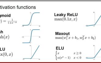
Activation functions play a crucial role in deep learning. They can introduce nonlinear characteristics into neural networks, allowing the network to better learn and simulate complex input-output relationships. The correct selection and use of activation functions has an important impact on the performance and training results of neural networks. This article will introduce four commonly used activation functions: Sigmoid, Tanh, ReLU and Softmax, starting from the introduction, usage scenarios, advantages, disadvantages and optimization solutions. Dimensions are discussed to provide you with a comprehensive understanding of activation functions. 1. Sigmoid function Introduction to SIgmoid function formula: The Sigmoid function is a commonly used nonlinear function that can map any real number to between 0 and 1. It is usually used to unify the
 Beyond ORB-SLAM3! SL-SLAM: Low light, severe jitter and weak texture scenes are all handled
May 30, 2024 am 09:35 AM
Beyond ORB-SLAM3! SL-SLAM: Low light, severe jitter and weak texture scenes are all handled
May 30, 2024 am 09:35 AM
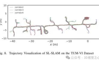
Written previously, today we discuss how deep learning technology can improve the performance of vision-based SLAM (simultaneous localization and mapping) in complex environments. By combining deep feature extraction and depth matching methods, here we introduce a versatile hybrid visual SLAM system designed to improve adaptation in challenging scenarios such as low-light conditions, dynamic lighting, weakly textured areas, and severe jitter. sex. Our system supports multiple modes, including extended monocular, stereo, monocular-inertial, and stereo-inertial configurations. In addition, it also analyzes how to combine visual SLAM with deep learning methods to inspire other research. Through extensive experiments on public datasets and self-sampled data, we demonstrate the superiority of SL-SLAM in terms of positioning accuracy and tracking robustness.
 Latent space embedding: explanation and demonstration
Jan 22, 2024 pm 05:30 PM
Latent space embedding: explanation and demonstration
Jan 22, 2024 pm 05:30 PM
Latent Space Embedding (LatentSpaceEmbedding) is the process of mapping high-dimensional data to low-dimensional space. In the field of machine learning and deep learning, latent space embedding is usually a neural network model that maps high-dimensional input data into a set of low-dimensional vector representations. This set of vectors is often called "latent vectors" or "latent encodings". The purpose of latent space embedding is to capture important features in the data and represent them into a more concise and understandable form. Through latent space embedding, we can perform operations such as visualizing, classifying, and clustering data in low-dimensional space to better understand and utilize the data. Latent space embedding has wide applications in many fields, such as image generation, feature extraction, dimensionality reduction, etc. Latent space embedding is the main
 Understand in one article: the connections and differences between AI, machine learning and deep learning
Mar 02, 2024 am 11:19 AM
Understand in one article: the connections and differences between AI, machine learning and deep learning
Mar 02, 2024 am 11:19 AM
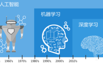
In today's wave of rapid technological changes, Artificial Intelligence (AI), Machine Learning (ML) and Deep Learning (DL) are like bright stars, leading the new wave of information technology. These three words frequently appear in various cutting-edge discussions and practical applications, but for many explorers who are new to this field, their specific meanings and their internal connections may still be shrouded in mystery. So let's take a look at this picture first. It can be seen that there is a close correlation and progressive relationship between deep learning, machine learning and artificial intelligence. Deep learning is a specific field of machine learning, and machine learning
 Super strong! Top 10 deep learning algorithms!
Mar 15, 2024 pm 03:46 PM
Super strong! Top 10 deep learning algorithms!
Mar 15, 2024 pm 03:46 PM
Almost 20 years have passed since the concept of deep learning was proposed in 2006. Deep learning, as a revolution in the field of artificial intelligence, has spawned many influential algorithms. So, what do you think are the top 10 algorithms for deep learning? The following are the top algorithms for deep learning in my opinion. They all occupy an important position in terms of innovation, application value and influence. 1. Deep neural network (DNN) background: Deep neural network (DNN), also called multi-layer perceptron, is the most common deep learning algorithm. When it was first invented, it was questioned due to the computing power bottleneck. Until recent years, computing power, The breakthrough came with the explosion of data. DNN is a neural network model that contains multiple hidden layers. In this model, each layer passes input to the next layer and
 From basics to practice, review the development history of Elasticsearch vector retrieval
Oct 23, 2023 pm 05:17 PM
From basics to practice, review the development history of Elasticsearch vector retrieval
Oct 23, 2023 pm 05:17 PM
1. Introduction Vector retrieval has become a core component of modern search and recommendation systems. It enables efficient query matching and recommendations by converting complex objects (such as text, images, or sounds) into numerical vectors and performing similarity searches in multidimensional spaces. From basics to practice, review the development history of Elasticsearch vector retrieval_elasticsearch As a popular open source search engine, Elasticsearch's development in vector retrieval has always attracted much attention. This article will review the development history of Elasticsearch vector retrieval, focusing on the characteristics and progress of each stage. Taking history as a guide, it is convenient for everyone to establish a full range of Elasticsearch vector retrieval.
 To provide a new scientific and complex question answering benchmark and evaluation system for large models, UNSW, Argonne, University of Chicago and other institutions jointly launched the SciQAG framework
Jul 25, 2024 am 06:42 AM
To provide a new scientific and complex question answering benchmark and evaluation system for large models, UNSW, Argonne, University of Chicago and other institutions jointly launched the SciQAG framework
Jul 25, 2024 am 06:42 AM
Editor |ScienceAI Question Answering (QA) data set plays a vital role in promoting natural language processing (NLP) research. High-quality QA data sets can not only be used to fine-tune models, but also effectively evaluate the capabilities of large language models (LLM), especially the ability to understand and reason about scientific knowledge. Although there are currently many scientific QA data sets covering medicine, chemistry, biology and other fields, these data sets still have some shortcomings. First, the data form is relatively simple, most of which are multiple-choice questions. They are easy to evaluate, but limit the model's answer selection range and cannot fully test the model's ability to answer scientific questions. In contrast, open-ended Q&A
