Excel function learning: Use summation function to calculate complex product costs

How to calculate the cost of finished products based on the cost of accessories. This problem seems a bit complicated, and I feel like I can't think of a good solution at once. In fact, it is very simple, and you can easily solve the problem using only a common summation function. Without further ado, let's take a look. Bar!

The problem I shared today came from a group friend’s request for help. Judging from his usual performance, this friend’s skills are quite good and he often helps other people in the group. His friends offered help, but when faced with his own problems, he seemed to have no solution.

In fact, I believe everyone can understand the problem he encountered at a glance. The problem is not too difficult to understand, but it seems that he doesn’t know how to solve it. The problem is as shown in the figure:

# is a type of problem for manufacturing companies to calculate product costs.

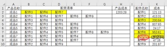
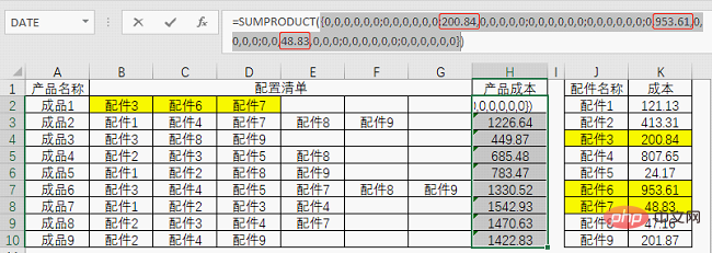
There are many kinds of accessories in the table. Different accessories are combined into finished products. The same accessories only appear once in a product. The current problem is to calculate the cost of the finished product based on the cost of the accessories. For example, the cost of finished product 1 is 200.84 953.61 48.83=1203.28.

I believe everyone can understand this calculation rule. In the actual environment, there are far more products and accessories than these 9 types. If you calculate them one by one manually, it will be inefficient and prone to errors.

So for such a problem, is there a formula that can help us get the correct result?

There must be, and there is more than one way.

Today I would like to share with you two formulas that are easier to understand.

Formula 1: SUM-SUMIF combination

The specific formula is=SUM(SUMIF($J$2:$J$10, B2:G2,$K$2:$K$10)), let’s take a look at the operation method.

This is an array formula. After inputting, you need to press Ctrl Shift Enter. Curly brackets will be automatically added on both sides of the formula to get the result.

The core part of the formula is of course SUMIF.

The difference from the basic usage is that in this example, the second parameter of SUMIF, that is, the condition for summation is an area:

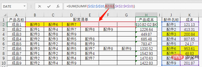
When seeking When the sum condition is multiple values ​​or multiple cells, SUMIF will get a set of data, and you can use the F9 key to see the result.

In layman’s terms, SUMIF calculates the cost corresponding to each accessory here, and then SUM completes the task of totaling the cost.

# Having said this, I believe everyone should understand the routine of this formula.

It can be seen that some seemingly troublesome problems can be solved by using some common functions as long as you find the right idea.

In fact, for this problem, using two functions is a bit redundant, and one SUMPRODUCT can easily solve it.

Formula 2: SUMPRODUCT function

The specific formula is: =SUMPRODUCT((B2:G2=$J$2:$J $10)*$K$2:$K$10), let’s see how it works.

This formula looks shorter than the first formula, but it is a little more difficult to understand. The formula uses logical values ​​and array calculation rules to achieve the final result.

(B2:G2=$J$2:$J$10)This part obtains a lot of logical values ​​by comparing each data in the configuration list and the accessory name list:

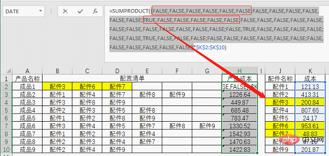
It seems densely packed, but if you look carefully, there are still certain regularities. For example, there is a semicolon between the six logical values. That is to say, the data in B2:G2 is first compared with J2. If there is no match, a set of FALSE is obtained, and then the data in B2:G2 is compared with J3. , and so on, until the process is completed when compared with J10.

The position pointed by the arrow indicates that in the third round of comparison, accessory 3 is matched, so a TRUE is obtained, and the same is true for the rest.

Although this bunch of logical values ​​may seem like a lot, the only ones that are actually useful are TRUE. Logical values ​​have a characteristic: FALSE is equal to 0 when calculated, and TRUE is equal to 1 when calculated. Multiplying the comparison by the area where the cost is located results in a set of numbers.

This makes it much clearer. The function of the SUMPRODUCT function is just to sum this set of numbers.

Related learning recommendations: excel tutorial

The above is the detailed content of Excel function learning: Use summation function to calculate complex product costs. For more information, please follow other related articles on the PHP Chinese website!