 Technology peripherals
 AI
AI
 Hinton's latest research: The future of neural networks is forward-forward algorithm
Hinton's latest research: The future of neural networks is forward-forward algorithm
In the past decade, deep learning has achieved amazing success, and the method of stochastic gradient descent with a large number of parameters and data has been proven to be effective. Gradient descent usually uses the backpropagation algorithm, so questions such as whether the brain follows backpropagation and whether there are other ways to obtain the gradients needed to adjust connection weights have always attracted much attention.
Turing Award winner and deep learning pioneer Geoffrey Hinton, as one of the proposers of backpropagation, has repeatedly proposed in recent years that backpropagation cannot explain how the brain works. . Instead, he is proposing a new neural network learning method - Forward-Forward Algorithm (FF).
At the recent NeurIPS 2022 conference, Hinton delivered a special speech titled "The Forward-Forward Algorithm for Training Deep Neural Networks", discussing the forward algorithm. Advantages compared to the reverse algorithm. The first draft of the paper "The Forward-Forward Algorithm: Some Preliminary Investigations" has been placed on the homepage of the University of Toronto:
##Paper Address: https://www.cs.toronto.edu/~hinton/FFA13.pdf
is different from the back propagation algorithm which uses one forward pass and one backward pass ,The FF algorithm consists of two forward passes, one ,using positive (i.e. real) data and the other using negative data ,generated by the network itself.Hinton believes that the advantage of the FF algorithm is that it can better explain the brain's cortical learning and can simulate hardware with extremely low power consumption.
Hinton advocates that the computer form that separates software and hardware should be abandoned. Future computers should be designed to be "non-mortal", thereby greatly saving computing resources, and # The ##FF algorithm is exactly the best learning method to run efficiently on this kind of hardware.
#This may be an ideal way to solve the computing power constraints of large models with trillions of parameters in the future.
1
FF algorithm is better at explaining the brain and more energy-saving than the reverse algorithm
In the FF algorithm, each layer has its own objective function, which has high goodness for positive data and low goodness for negative data. The activity sum of squares in a layer can be used as a measure of goodness, and many other possibilities are included, such as subtracting the activity sum of squares.If positive and negative passes can be separated in time, negative passes can be completed offline, learning of positive passes will be simpler, and allow videos to be transmitted over the network without storing activity or termination propagation derivatives.
Hinton believes that the FF algorithm is better than backpropagation in two aspects:
First, FF is to explain cerebral cortex learning A better model;
Second, FF is more energy-efficient,
It uses extremely low-power simulation hardware without resorting to reinforcement learning.There is no tangible evidence that the cortex propagates error derivatives or stores neural activity for subsequent backpropagation. Top-down connections from one cortical area to areas earlier in the visual pathway do not reflect the bottom-up connections expected when backpropagation is used in the visual system. Instead, they form loops in which neural activity passes through two areas, about six cortices, and then returns to where it started.
As one of the ways to learn sequences, the credibility of backpropagation through time is not high. To process a stream of sensory input without frequent pauses, the brain needs to transmit data through the different stages of sensory processing and also needs a process that can learn on the fly. Representations later in the pipeline may provide top-down information later in time that affects representations in earlier stages of the pipeline, but the perceptual system needs to reason and learn in real time, rather than stalling for backpropagation.
Another serious limitation of backpropagation is that it requires complete understanding of the calculations performed by forward propagation in order to derive the correct derivatives. If we insert a black box in forward propagation, backpropagation cannot be performed unless a differentiable model of the black box is learned.
The black box will not affect the learning process of the FF algorithm, because there is no need to perform backpropagation through it.
When there is no perfect forward propagation model, we can start from a variety of reinforcement learning methods. One idea is to perform random perturbations on weights or neural activity and correlate these perturbations with the resulting changes in the payoff function. However, due to the high variance problem in reinforcement learning: when other variables are perturbed at the same time, it is difficult to see the effect of perturbing a single variable. To do this, to average out the noise caused by all other perturbations, the learning rate needs to be inversely proportional to the number of variables being perturbed, which means that reinforcement learning scales poorly to large networks containing millions or billions. backpropagation competition parameters.
And Hinton’s point is that neural networks containing unknown nonlinearities do not need to resort to reinforcement learning.
The FF algorithm is comparable to backpropagation in speed. Its advantage is that it can be used when the precise details of the forward calculation are unknown, and it can also be used in neural networks. Learning occurs while pipeline processing on sequential data without the need to store neural activity or terminate propagation error derivatives.
However, in power-constrained applications, the FF algorithm has not yet replaced backpropagation. For example, for very large models trained on very large data sets, it is still possible to Mainly backpropagation.
Forward-forward algorithm
Forward-forward algorithm is a greedy multi-layer learning procedure inspired by Glass Oltzmann machines and noise contrastive estimation.
Replace the forward and backward passes of backpropagation with two forward passes that operate on different data and opposite targets, operating in exactly the same way as each other. Among them, the forward channel operates on real data and adjusts the weights to increase the favorability of each hidden layer, and the reverse channel adjusts the "negative data" weights to reduce the favorability of each hidden layer.
This article explores two different metrics - the sum of the squares of neural activity, and the sum of the squares of negative activity.
Assume that the goodness function of a certain layer is the sum of squares of the rectified linear neuron activities in the layer, and the purpose of learning is to make its goodness much higher than a certain threshold of the real data , and well below the threshold of negative data. That is, the probability that an input vector is positive (i.e., true) when it is correctly classified as positive or negative data can be determined by applying the logistic function σ to the goodness-of-goodness minus some threshold θ:

Where,  is the activity of hidden unit j before layer normalization. Negative data can be predicted by top-down connections of neural networks or provided externally.
Learning multi-layer representations using layer-by-layer optimization functions
It is easy to see that the alignment can be achieved by making the sum of the squares of the activities of the hidden units High for data and low for negative data to learn a single hidden layer. But when the first hidden layer activity is used as the input of the second hidden layer, only the activity vector length of the first hidden layer is applied to distinguish positive and negative data without learning new features.
To prevent this situation, FF will normalize the hidden vector length before using it as the input of the next layer, and delete all the information used to determine the first hidden layer. information in the first hidden layer, thus forcing the next hidden layer to use the relative activity information of the neurons in the first hidden layer, which is not affected by layer normalization.
That is to say, The activity vector of the first hidden layer has a length and a direction. The length is used to define the benignity of the layer, and only the direction is passed to the next layer.
2
Experiments on FF algorithm
Backpropagation baseline
Most of the experiments in this article used the MNIST dataset of handwritten digits: 50,000 for training, 10,000 for validation during the search for good hyperparameters, and 10,000 for calculating the test error rate. A convolutional neural network designed with several hidden layers can achieve a test error of about 0.6%.
In the "arrangement-invariant" version of the task, the neural network does not get information about the spatial layout of the pixels. If before training starts, all training and test images are affected by the random mutation of the same pixels. , then the neural network will perform equally well.
For the "permutation invariant" version of this task, the test error of a feedforward neural network with a rectified linear unit (ReLU) with several fully connected hidden layers is approximately 1.4%, where It takes about 20 epochs to train. Using various regularizers such as dropout (which slows down training) or label smoothing (which speeds up training), the test error can be reduced to around 1.1%. In addition, the test error can be further reduced by combining supervised learning of labels with unsupervised learning.
Without using complex regularizers, the “permutation-invariant” version of the task achieved a test error of 1.4%, demonstrating that the learning process is as effective as backpropagation .

Figure 1: Mixed image used as negative data
None Supervised FF Algorithm
FF There are two main questions to answer: Given a good source of negative data, will it learn an efficient multi-layer representation to capture the data structure? Where do negative data come from?
First use manual negative data to answer the first question. A common way to use contrastive learning for supervised learning tasks is to transform the input vectors into representation vectors without using any information about the labels, and learn to simply linearly transform these representation vectors into logits vectors using, in softmax, to determine the probability distribution of labels. Despite the obvious non-linearity, this is still called a linear classifier, where the learning of the linear transformation of the logits vector is supervised, since it does not involve learning any hidden layers and no backpropagation of derivatives is required. FF can perform this representation learning by using real data vectors as positive examples and corrupted data vectors as negative examples.
To make FF focus on characterizing the long-term correlation of shape images, we need to create negative data with different long-term correlations, but very similar short-term correlations. This can be done by creating a Complete with a fairly large mask of 1's and 0's areas. A hybrid image is then created for negative data by adding a digital image to the mask and a different digital image to multiply the opposite side of the mask (Figure 1).
Start creating a mask from a random bitmap, and blur the image repeatedly using filters of the form [1/4, 1/2, 1/4] in both horizontal and vertical directions. The threshold for repeatedly blurred images was set to 0.5. After training for 100 epochs using four hidden layers (each hidden layer contains 2000 ReLU), if the normalized activity vectors of the last three hidden layers are used as softmax input, the test error is 1.37%.
In addition, not using fully connected layers but using local receptive fields (without weight sharing) can improve performance. The test error of training for 60 epochs is 1.16%. The architecture uses " Peer Normalization" prevents any hidden unit from becoming hyperactive or permanently shut down.
Supervised learning FF algorithm
Learns hidden representations without using any label information, which may eventually be able to perform various tasks Very sensible for large models: unsupervised learning extracts a large set of features for each task. But if you are only interested in a single task and want to use a small model, then supervised learning will be more suitable.
One way to use FF in supervised learning is to include labels in the input. Positive data consists of images with correct labels, while negative data consists of images with incorrect labels. The label is the only one between the two. The difference is that FF ignores all features in the image that are not relevant to the label.
MNIST images contain black borders to ease the work of convolutional neural networks. The first hidden layer learning content is also easily revealed when replacing the first 10 pixels with one of the N representations of the label. In a network with 4 hidden layers, each hidden layer contains 2000 ReLUs. After 60 epochs, the complete connection between layers has a test error of 1.36% by MNIST. Backpropagation is required to achieve this test performance. About 20 epochs. Doubling the FF learning rate and training for 40 epochs results in a slightly worse test error of 1.46%.
After training with FF, the test digits are classified by making a forward pass by the network starting from an input containing the test digit and a neutral label consisting of 10 0.1 entries ,After that, all hidden activities except the first hidden layer are used as ,softmax inputs learned during training, which is a fast ,suboptimal method for image classification. The best way is to run the network with a specific label as part of the input and accumulate the merits of all layers except the first hidden layer. After doing this for each label separately, choose the label with the highest cumulative merit. . During training, the forward pass from neutral labels is used to pick out hard negative labels, which makes training require about ⅓ of the epochs.
The two most dithered pixels of the image in each direction are used to increase the training data, thereby obtaining 25 different offsets for each image, using pixel space layout knowledge, so that it is no longer an invariant arrangement. By training the same network with augmented data for 500 epochs, the test error can reach 0.64%, similar to a convolutional neural network trained with backpropagation. As shown in Figure 2, we also get interesting local domains in the first hidden layer.
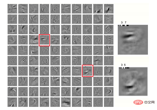
Figure 2: Local domain, class label, of 100 neurons in the first hidden layer of a network trained on jittered MNIST Displayed in the first 10 pixels of each image
Use FF to simulate top-down perceptual effects
Currently, all The image classification examples all use feedforward neural networks that learn one layer at a time, which means that what is learned in later layers does not affect the learning of previous layers. This seems to be a major weakness compared to backpropagation, and the key to overcoming this apparent limitation is to treat static images as rather boring videos, processed by multi-layer recurrent neural networks.
FF Both positive and negative data run forward in time, but the activity vector of each layer is normalized by the previous time-steps of the previous layer and the next layer. The activity vector is determined (Figure 3). As a preliminary check whether this approach works, one can use a "video" input consisting of a static MNIST image that is simply repeated in each time frame, with a pixel image at the bottom and one of N representations of the numeric class at the top, There are two or three intermediate layers, each with 2000 neurons.
In preliminary experiments, the recurrent network ran for 10 time-steps. The even-numbered layers of each time-steps were updated according to the normalization activities of the odd-numbered layers, and the odd-numbered layers were updated according to the new normalization. Activity updates, whose alternating updates are designed to avoid biphasic oscillations, but currently don't seem to be : synchronization of all hidden layers based on the previous time-steps normalized state with a little damping Update learning is slightly better, which is beneficial for irregular architectures. Therefore, synchronous updates were used in this experiment, and the new pre-normalized state was set to 0.3 of the previous pre-normalized state, plus 0.7 of the calculated new state.
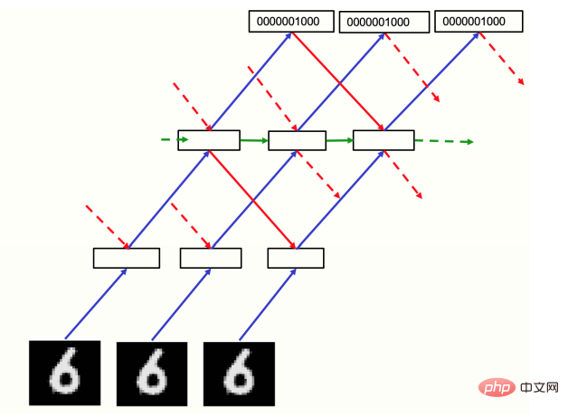
Figure 3: Recurrent network for processing video
As Figure 3. The network is trained on MNIST for 60 epochs, and the hidden layer of each image is initialized in a bottom-up pass.
Thereafter, the network runs 8 synchronous iterations with damping, by running 8 iterations for each of the 10 labels and selecting the label with the highest average goodness in iterations 3 to 5 To evaluate the test data performance of the network, the test error is 1.31%. Negative data are passed forward through the network once to obtain the probabilities of all categories, and incorrect categories are selected and generated in proportion to the probabilities, thereby improving training efficiency.
Prediction using spatial context
In a recurrent network, the goal is to maintain a good relationship between the upper layer input of positive data and the input of the lower layer. Consistency, while the consistency of negative data is not good. A desirable property in a network with spatially local connectivity: the top-down input will be determined by a larger area of the image and have the result of more processing stages, so it can be viewed as a contextual prediction of the image, as well. That is the result that should be produced based on the bottom-up input of the local image domain.
If the input changes over time, the top-down input will be based on older input data, so representations that predict the bottom-up input must be learned. When we reverse the sign of the objective function and perform a low-squared activity for positive data, the top-down input should learn to cancel out the bottom-up input for positive data, which appears to be very similar to predictive coding. Layer normalization means that even if cancellation works well, a lot of information is sent to the next layer, which is amplified by normalization if all prediction errors are small.
The idea of using context predictions as local features and extracting teaching signals for learning has been around for a long time, but the difficulty lies in how to work in neural networks that use spatial context rather than unilateral temporal context. Using consensus from top-down and bottom-up inputs as teaching signals for top-down and bottom-up weights is an approach that clearly leads to collapse, as is the problem of using contextual predictions from other images to create negative pairs. Not completely resolved. Among them, using negative data rather than any negative internal representation seems to be the key.
CIFAR-10 data set test
Hinton then tested the performance of the FF algorithm on the CIFAR‑10 data set, proving that FF training The resulting network is comparable in performance to backpropagation.
The dataset has 50,000 32x32 training images with three color channels per pixel, so each image has 3072 dimensions. Since the background of these images is complex and highly variable and cannot be modeled well with very limited training data, a fully connected network containing two to three hidden layers can be used using backpropagation unless the hidden layer is very small. There will be severe overfitting when training, so almost all current research results are for convolutional networks.
Backpropagation and FF both use weight decay to reduce overfitting. Hinton compared the performance of the networks trained by the two methods. For the FF-trained network, the test method is to use a single forward propagation, or have the network run 10 iterations on the image and each of the 10 labels, and accumulate the energy of the label in iterations 4 to 6 (i.e., when based on when the goodness of error is lowest).
As a result, although the test performance of FF is worse than backpropagation, it is only slightly worse. At the same time, the gap between the two will not increase with the increase of hidden layers. However, backpropagation can reduce training error faster.
In addition, in sequence learning, Hinton also proved that the network trained with FF is better than backpropagation through the task of predicting the next character in the sequence. Networks trained with FF can generate their own negative data and are more biologically consistent.
3
The relationship between FF algorithm and Boltzmann machine, GAN, SimCLR
Hinton further developed the FF algorithm It is compared with other existing contrastive learning methods. His conclusion is:
FF is a combination of Boltzmann machines and simple local goodness functions;
FF is not required Back propagation is used to learn the discriminative model and the generative model, so it is a special case of GAN;
In real neural networks, compared with self-supervised comparison methods such as SimCLR, FF can Better measure of consistency between two different representations.
FF absorbs the contrastive learning of Boltzmann machines
In the early 1980s, deep neural networks had two of the most promising learning methods, one It is backpropagation, and the other is Boltzmann Machines that do unsupervised comparative learning.
A Boltzmann machine is a network of stochastic binary neurons with pairwise connections with equal weights in both directions. When it is free to run without external input, the Boltzmann machine repeatedly updates each binary neuron by setting it to the on state with probability equal to the total input it receives from other active neurons. logic. This simple update process ultimately samples from an equilibrium distribution, where each global configuration (which assigns a binary state to all neurons) has a log probability proportional to its negative energy. Negative energy is simply the sum of the weights between all pairs of neurons in that configuration.
A subset of neurons in a Boltzmann machine is "visible", binary data vectors are presented to the network by clamping them over the visible neurons, and then letting it update repeatedly The remaining hidden neuron states. The purpose of Boltzmann machine learning is to make the distribution of binary vectors on visible neurons freely match the data distribution when the network is running.
The most surprising thing is that when the free-running Boltzmann machine is in thermal equilibrium, the Kullback-Liebler divergence between the data distribution displayed on the neurons and the model distribution can be seen has a very simple derivative (for any weight):

where the angle brackets indicate the expectation of random fluctuations at thermal equilibrium and the data for the first term .
What is exciting about this result is that it gives the derivatives of the weights deep in the network without explicitly propagating the error derivatives. It spreads neural activity during two different stages of wakefulness and sleep.
However, the cost of making the learning rules the simplest mathematically is very high. It requires a deep Boltzmann machine to approximate its equilibrium distribution, which makes it unrealistic as a machine learning technique and implausible as a cortical learning model: large networks do not have time to approximate its equilibrium distribution during perception. Balanced distribution. Moreover, there is no evidence for detailed symmetry of cortical connections, nor an obvious way to learn sequences. Furthermore, Boltzmann machine learning procedures will fail if many positive updates of weights are followed by many negative updates, and the negative phase corresponds to REM sleep.
But despite the above shortcomings, the Boltzmann machine is still a very smart learning method because it uses two working principles that work the same but have different boundaries on the visible neurons. Iterative setting of conditions (i.e., restricted on data vs. unrestricted), replaces the forward and backward passes of backpropagation.
The Boltzmann machine can be seen as a combination of two ideas:
- By minimizing the freedom on real data (free energy) and maximize the free energy on negative data to learn the data generated by the network itself.
- Uses the Hopfield energy as the energy function and uses repeated random updates to sample the global configuration from a Boltzmann distribution defined by the energy function.
The first idea about contrastive learning can be used with many other energy functions. For example, the output of a feedforward neural network is used to define the energy, and then backpropagation is used through the network to calculate the derivative of the energy with respect to the weights and visible states. Negative data is then generated by tracking the derivative of the energy with respect to the visible state. In addition, negative data does not have to be generated by sampling data vectors from the Boltzmann distribution defined by the energy function, which can also improve the learning efficiency of Boltzmann machines with a single hidden layer without sampling from the equilibrium distribution.
In Hinton's view, the mathematical simplicity of Equation 2 and the stochastic update process of doing Bayesian integration over all possible hidden configurations are really elegant, so using only The idea that two solutions for propagating neural activity are needed instead of forward backpropagation for backpropagation is still entangled with the complexities of Markov Chain Monte Carlo.
Simple local goodness functions are easier to handle than the free energy of binary random neuron networks, and FF combines the contrastive learning of Boltzmann machines with this function.
FF is a special case of GAN
GAN (Generative Adversarial Network) uses a multi-layer neural network to generate data and uses multiple layers The discriminative network trains its generative model to give a derivative with respect to the generative model output, and the probability that the derivative is real data rather than generated data
GAN is difficult to train because the discriminant Models and generative models are pitted against each other. GANs can produce very beautiful images, but they suffer from mode collapse: there can be large regions of image space that never generate examples. And it uses backpropagation to fit each network, so it's hard to see how to implement them in cortex.
FF can be regarded as a special case of GAN, in which each hidden layer of the discriminant network will make its own greedy decision on the positive or negative input, so there is no need for backpropagation To learn the discriminative model and the generative model, because it does not learn its own hidden representation, but reuses the representation learned by the discriminative model.
The only thing a generative model needs to learn is how to transform these hidden representations into generated data. If a linear transformation is used to calculate the logarithm of the softmax, no backpropagation is needed. One advantage of using the same hidden representation for both models is that it eliminates the problems that arise when one model learns too quickly relative to the other, and also avoids mode collapse.
FF is easier to measure consistency than SimCLR
Self-supervised comparison methods like SimCLR learn by optimizing an objective function. This function is able to support consistency between representations of two different crops of the same image, as well as inconsistency between representations of crops from two different images.
This type of method usually uses many layers to extract the clipped representation and trains these layers by backpropagating the derivative of the objective function. They don't work if the two clippings always overlap in the exact same way, because then they can simply report the intensity of the shared pixels and get perfect consistency.
But in a real neural network, it is not easy to measure the consistency between two different representations, and there is no way to extract two clipped representations at the same time using the same weights.
And FF uses a different way to measure consistency, which seems easier for real neural networks.
Many different sources of information provide input to the same group of neurons. If the sources agree on which neurons to activate, there will be positive interference, resulting in high squared activity, and if they disagree, the squared activity will be low. Measuring consistency by using positive interference is much more flexible than comparing two different representation vectors because there is no need to arbitrarily split the input into two separate sources.
SimCLR A major weakness of this type of approach is the large amount of computation used to derive a representation of the two image crops, but the objective function only provides modest constraints on the representation, which limits the domain in question. The rate of information can inject weight. In order for the clipped representation to be closer to its correct pair than to a substitute, only 20 bits of information are required. The problem with FF is more severe because it only requires 1 bit to distinguish between positive and negative examples.
The solution to this poverty of constraints is to split each layer into many small blocks and force each block to use the length of its pre-normalized activity vector to decide the positive and Negative example. The information required to satisfy the constraints then scales linearly with the number of blocks, which is much better than the logarithmic scaling achieved with larger contrast sets in SimCLR-like methods.
Problems in stack contrast learning
An unsupervised method for learning multi-layer representation is to first learn a hidden layer, which A layer captures some structure in the data, then the activity vectors in that layer are treated as data and the same unsupervised learning algorithm is applied again. This is how multi-layer representations are learned using restricted Boltzmann machines (RBMs) or stacked autoencoders.
But it has a fatal flaw. Suppose we map some random noise images through a random weight matrix. The resulting activity vector will have a correlation structure created by the weight matrix, independent of the data. When unsupervised learning is applied to these activity vectors, it discovers some structure within them, but this does not tell the system anything about the outside world.
The original Boltzmann machine learning algorithm was designed to avoid this flaw by comparing statistics caused by two different external boundary conditions. This cancels out any structure that is simply a result of other parts of the network. There is no need to constrain routing when comparing positive and negative data, nor does it require random spatial relationships between clippings to prevent network cheating. This makes it easy to obtain a large number of interconnected neuron groups, each with its own goal of distinguishing positive data from negative data.
4
On future non-immortal computers
FF is the best learning algorithm
Mortal Computation is one of Hinton's recent important views (note: this term does not have a recognized Chinese translation, and is tentatively translated as "non-immortal computation").
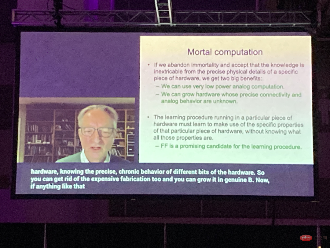
# He pointed out that current general-purpose digital computers are designed to faithfully follow instructions, and it is believed that the only way to get a general-purpose computer to perform a specific task is to Write a program that specifies exactly what to do in an extremely detailed way.
The mainstream thinking still insists that software should be separated from hardware so that the same program or the same set of weights can run on different physical copies of the hardware. This makes the knowledge contained in the program or weights "immortal": when the hardware dies, the knowledge does not die with it.
But this is no longer true, and the research community has yet to fully understand the long-term impact of deep learning on the way computers are built.
The separation of software and hardware is one of the foundations of computer science. It does bring many benefits, such as the ability to study the characteristics of a program without having to care about electrical engineering, and it makes writing once program and copy it to millions of computers. But Hinton points out:
#If we are willing to give up this "immortality," we can save significantly the energy required to perform the calculations and the cost of manufacturing the hardware to perform the calculations.
In this way, different hardware instances performing the same task may have large changes in connectivity and nonlinearity, and effective utilization can be found from the learning process Parameter values for unknown properties of each specific instance of hardware. These parameter values are only useful for a specific hardware instance, so the calculations they perform are not immortal and will perish with the hardware.
Copying parameter values to different hardware that works differently doesn't really make sense in itself, but we can use a more biological approach to transfer what one piece of hardware has learned to Another piece of hardware. For a task like object classification in an image, what we are really interested in is the function that relates pixel intensity to the class label, not the parameter values that implement that function in a particular hardware.
The function itself can be transferred to different hardware by using distillation: training new hardware not only gives the same answers as the old hardware, but also outputs the same probability for incorrect answers. These probabilities give a richer indication of how the old model generalized, rather than just what labels it thought were most likely. So by training the new model to match the probability of wrong answers, we are training it to generalize in the same way as the old model. It is a rare example of such a neural network training actually optimizing generalization.
If you want a trillion-parameter neural network to consume only a few watts, non-immortal computing may be the only option. Its feasibility depends on whether we can find a learning process that can run efficiently in hardware whose precise details are unknown. In Hinton’s view, FF algorithm is a promising solution, but it How it performs when scaling to large neural networks remains to be seen.
At the end of the paper, Hinton points out the following open questions:
- Can FF generate good enough image or video generative models to create the tools for unsupervised learning? Need negative data?
- If negative passes are completed during sleep, can positive and negative passes be very broadly distinguished in time?
- If the negative phase was eliminated for a period of time, would the effect be similar to the damaging effects of severe sleep deprivation?
- Which goodness function is best to use? This paper uses the activity sum of squares in most experiments, but minimizing the activity sum of squares for positive data and maximizing the activity sum of squares for negative data seems to work slightly better.
- Which activation function is best to use? Only ReLU has been studied so far. Making the activation be the negative logarithm of the density under the t-distribution is one possibility.
- For spatial data, can FF benefit from a large number of local optimization functions in different areas of the image? If it works, it speeds up learning.
- For sequential data, is it possible to use fast weights to simulate a simplified transformer?
- A set of features that try to maximize their squared activity Can FF be supported by a detector and a set of constraint violation detectors that try to minimize their squared activity?
The above is the detailed content of Hinton's latest research: The future of neural networks is forward-forward algorithm. For more information, please follow other related articles on the PHP Chinese website!

Hot AI Tools

Undresser.AI Undress
AI-powered app for creating realistic nude photos

AI Clothes Remover
Online AI tool for removing clothes from photos.

Undress AI Tool
Undress images for free

Clothoff.io
AI clothes remover

Video Face Swap
Swap faces in any video effortlessly with our completely free AI face swap tool!

Hot Article

Hot Tools

Notepad++7.3.1
Easy-to-use and free code editor

SublimeText3 Chinese version
Chinese version, very easy to use

Zend Studio 13.0.1
Powerful PHP integrated development environment

Dreamweaver CS6
Visual web development tools

SublimeText3 Mac version
God-level code editing software (SublimeText3)

Hot Topics
 1387
1387
 52
52
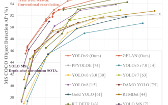 YOLO is immortal! YOLOv9 is released: performance and speed SOTA~
Feb 26, 2024 am 11:31 AM
Today's deep learning methods focus on designing the most suitable objective function so that the model's prediction results are closest to the actual situation. At the same time, a suitable architecture must be designed to obtain sufficient information for prediction. Existing methods ignore the fact that when the input data undergoes layer-by-layer feature extraction and spatial transformation, a large amount of information will be lost. This article will delve into important issues when transmitting data through deep networks, namely information bottlenecks and reversible functions. Based on this, the concept of programmable gradient information (PGI) is proposed to cope with the various changes required by deep networks to achieve multi-objectives. PGI can provide complete input information for the target task to calculate the objective function, thereby obtaining reliable gradient information to update network weights. In addition, a new lightweight network framework is designed
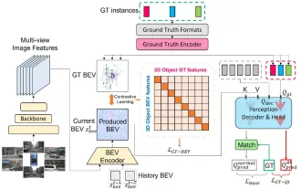 CLIP-BEVFormer: Explicitly supervise the BEVFormer structure to improve long-tail detection performance
Mar 26, 2024 pm 12:41 PM
Written above & the author’s personal understanding: At present, in the entire autonomous driving system, the perception module plays a vital role. The autonomous vehicle driving on the road can only obtain accurate perception results through the perception module. The downstream regulation and control module in the autonomous driving system makes timely and correct judgments and behavioral decisions. Currently, cars with autonomous driving functions are usually equipped with a variety of data information sensors including surround-view camera sensors, lidar sensors, and millimeter-wave radar sensors to collect information in different modalities to achieve accurate perception tasks. The BEV perception algorithm based on pure vision is favored by the industry because of its low hardware cost and easy deployment, and its output results can be easily applied to various downstream tasks.
 Implementing Machine Learning Algorithms in C++: Common Challenges and Solutions
Jun 03, 2024 pm 01:25 PM
Common challenges faced by machine learning algorithms in C++ include memory management, multi-threading, performance optimization, and maintainability. Solutions include using smart pointers, modern threading libraries, SIMD instructions and third-party libraries, as well as following coding style guidelines and using automation tools. Practical cases show how to use the Eigen library to implement linear regression algorithms, effectively manage memory and use high-performance matrix operations.
 Explore the underlying principles and algorithm selection of the C++sort function
Apr 02, 2024 pm 05:36 PM
The bottom layer of the C++sort function uses merge sort, its complexity is O(nlogn), and provides different sorting algorithm choices, including quick sort, heap sort and stable sort.
 1.3ms takes 1.3ms! Tsinghua's latest open source mobile neural network architecture RepViT
Mar 11, 2024 pm 12:07 PM
Paper address: https://arxiv.org/abs/2307.09283 Code address: https://github.com/THU-MIG/RepViTRepViT performs well in the mobile ViT architecture and shows significant advantages. Next, we explore the contributions of this study. It is mentioned in the article that lightweight ViTs generally perform better than lightweight CNNs on visual tasks, mainly due to their multi-head self-attention module (MSHA) that allows the model to learn global representations. However, the architectural differences between lightweight ViTs and lightweight CNNs have not been fully studied. In this study, the authors integrated lightweight ViTs into the effective
 Can artificial intelligence predict crime? Explore CrimeGPT's capabilities
Mar 22, 2024 pm 10:10 PM
The convergence of artificial intelligence (AI) and law enforcement opens up new possibilities for crime prevention and detection. The predictive capabilities of artificial intelligence are widely used in systems such as CrimeGPT (Crime Prediction Technology) to predict criminal activities. This article explores the potential of artificial intelligence in crime prediction, its current applications, the challenges it faces, and the possible ethical implications of the technology. Artificial Intelligence and Crime Prediction: The Basics CrimeGPT uses machine learning algorithms to analyze large data sets, identifying patterns that can predict where and when crimes are likely to occur. These data sets include historical crime statistics, demographic information, economic indicators, weather patterns, and more. By identifying trends that human analysts might miss, artificial intelligence can empower law enforcement agencies
 Improved detection algorithm: for target detection in high-resolution optical remote sensing images
Jun 06, 2024 pm 12:33 PM
01 Outlook Summary Currently, it is difficult to achieve an appropriate balance between detection efficiency and detection results. We have developed an enhanced YOLOv5 algorithm for target detection in high-resolution optical remote sensing images, using multi-layer feature pyramids, multi-detection head strategies and hybrid attention modules to improve the effect of the target detection network in optical remote sensing images. According to the SIMD data set, the mAP of the new algorithm is 2.2% better than YOLOv5 and 8.48% better than YOLOX, achieving a better balance between detection results and speed. 02 Background & Motivation With the rapid development of remote sensing technology, high-resolution optical remote sensing images have been used to describe many objects on the earth’s surface, including aircraft, cars, buildings, etc. Object detection in the interpretation of remote sensing images
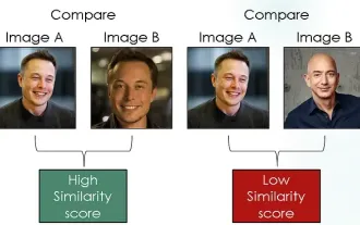 Exploring Siamese networks using contrastive loss for image similarity comparison
Apr 02, 2024 am 11:37 AM
Introduction In the field of computer vision, accurately measuring image similarity is a critical task with a wide range of practical applications. From image search engines to facial recognition systems and content-based recommendation systems, the ability to effectively compare and find similar images is important. The Siamese network combined with contrastive loss provides a powerful framework for learning image similarity in a data-driven manner. In this blog post, we will dive into the details of Siamese networks, explore the concept of contrastive loss, and explore how these two components work together to create an effective image similarity model. First, the Siamese network consists of two identical subnetworks that share the same weights and parameters. Each sub-network encodes the input image into a feature vector, which


