Summary of six common methods of continuous learning: adapting ML models to new data while maintaining the performance of old data

Continuous learning refers to a model that learns a large number of tasks sequentially without forgetting the knowledge gained from previous tasks. This is an important concept because, under supervised learning, machine learning models are trained to be the best function for a given data set or data distribution. In real-life environments, data is rarely static and may change. Typical ML models can suffer performance degradation when faced with unseen data. This phenomenon is called catastrophic forgetting.

#A common way to solve this type of problem is to retrain the entire model on a new, larger dataset containing both old and new data. But this approach is often costly. So there is a field of ML research that is looking into this problem, and based on the research in this field, this article will discuss 6 methods that allow the model to adapt to new data while maintaining the performance of the old, and avoid the need to train on the entire data set (old new) Retrain.

Prompt

Prompt The idea stems from the idea that hints (short sequences of words) for GPT 3 can help drive models to reason and answer better. So Prompt is translated as prompt in this article. Hint tuning refers to using small learnable hints and feeding them as input to the model along with real inputs. This allows us to only train a small model that provides hints on new data without having to retrain the model weights.

Specifically, I chose the example of using prompts for text-based intensive retrieval, which was adapted from Wang's article "Learning to Prompt for continuous Learning".

The authors of the paper describe their idea using the following diagram:

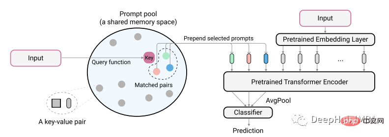
The actual encoded text input is used to identify the minimum matching pair from the prompt pool key. These identified cues are first added to unencoded text embeddings before they are fed into the model. The purpose of this is to train these cues to represent new tasks while keeping the old model unchanged. The cues here are very small, maybe only 20 tokens per prompt.

class PromptPool(nn.Module):
def __init__(self, M = 100, hidden_size = 768, length = 20, N=5):
super().__init__()
self.pool = nn.Parameter(torch.rand(M, length, hidden_size), requires_grad=True).float()
self.keys = nn.Parameter(torch.rand(M, hidden_size), requires_grad=True).float()
 
self.length = length
self.hidden = hidden_size
self.n = N
 
nn.init.xavier_normal_(self.pool)
nn.init.xavier_normal_(self.keys)
 
def init_weights(self, embedding):
pass
 
# function to select from pool based on index
def concat(self, indices, input_embeds):
subset = self.pool[indices, :] # 2, 2, 20, 768
 
subset = subset.to("cuda:0").reshape(indices.size(0),
self.n*self.length,
self.hidden) # 2, 40, 768
 
return torch.cat((subset, input_embeds), 1)
 
# x is cls output
def query_fn(self, x):
 
# encode input x to same dim as key using cosine
x = x / x.norm(dim=1)[:, None]
k = self.keys / self.keys.norm(dim=1)[:, None]
 
scores = torch.mm(x, k.transpose(0,1).to("cuda:0"))
 
# get argmin
subsets = torch.topk(scores, self.n, 1, False).indices # k smallest
 
return subsets
 
 pool = PromptPool()

Then we use the trained old data model to train new data. Here we only train the weight of the prompt part.

def train():
count = 0
print("*********** Started Training *************")
 
start = time.time()
for epoch in range(40):
model.eval()
pool.train()
 
optimizer.zero_grad(set_to_none=True)
lap = time.time()
 
for batch in iter(train_dataloader):
count += 1
q, p, train_labels = batch
 
queries_emb = model(input_ids=q['input_ids'].to("cuda:0"),
attention_mask=q['attention_mask'].to("cuda:0"))
passage_emb = model(input_ids=p['input_ids'].to("cuda:0"),
attention_mask=p['attention_mask'].to("cuda:0"))
 
# pool
q_idx = pool.query_fn(queries_emb)
raw_qembedding = model.model.embeddings(input_ids=q['input_ids'].to("cuda:0"))
q = pool.concat(indices=q_idx, input_embeds=raw_qembedding)
 
p_idx = pool.query_fn(passage_emb)
raw_pembedding = model.model.embeddings(input_ids=p['input_ids'].to("cuda:0"))
p = pool.concat(indices=p_idx, input_embeds=raw_pembedding)
 
qattention_mask = torch.ones(batch_size, q.size(1))
pattention_mask = torch.ones(batch_size, p.size(1))
 
queries_emb = model.model(inputs_embeds=q,
attention_mask=qattention_mask.to("cuda:0")).last_hidden_state
passage_emb = model.model(inputs_embeds=p,
attention_mask=pattention_mask.to("cuda:0")).last_hidden_state
 
q_cls = queries_emb[:, pool.n*pool.length+1, :]
p_cls = passage_emb[:, pool.n*pool.length+1, :]
 
loss, ql, pl = calc_loss(q_cls, p_cls)
loss.backward()
 
optimizer.step()
optimizer.zero_grad(set_to_none=True)
 
if count % 10 == 0:
print("Model Loss:", round(loss.item(),4), 
"| QL:", round(ql.item(),4), "| PL:", round(pl.item(),4), 
"| Took:", round(time.time() - lap), "secondsn")
 
lap = time.time()
 
if count % 40 == 0 and count > 0:
print("model saved")
torch.save(model.state_dict(), model_PATH)
torch.save(pool.state_dict(), pool_PATH)
 
if count == 4600: return
 
print("Training Took:", round(time.time() - start), "seconds")
print("n*********** Training Complete *************")

After training is completed, the subsequent inference process needs to combine the input with the retrieved hints. For example, this example got performance -93% for the new data hint pool, and -94% for full (old-new) training. This is similar to the performance mentioned in the original paper. But the caveat is that results may vary depending on the task, and you should try experiments to know what works best.

For this method to be worth considering, it must be able to preserve >80% of the performance of the old model on old data, while the hints should also help the model achieve good performance on new data.

The disadvantage of this method is that it requires the use of a hint pool, which adds extra time. This is not a permanent solution, but it is feasible for now, and perhaps new methods will emerge in the future.

Data Distillation

You may have heard of the term knowledge distillation, which is a technique that uses weights from a teacher model to guide and train smaller-scale models. Data Distillation works similarly, using weights from real data to train smaller subsets of the data. Because the key signals of the data set are refined and condensed into smaller data sets, our training on new data only needs to be provided with some refined data to maintain the old performance.

In this example, I apply data distillation to a dense retrieval (text) task. No one else is currently using this method in this field, so the results may not be the best, but if you use this method on text classification you should get good results.

Essentially, the idea of ​​text data distillation originated from a paper by Li titled Data Distillation for Text Classification, which was inspired by Wang's Dataset Distillation, where he distilled image data. Li describes the task of text data distillation with the following diagram:

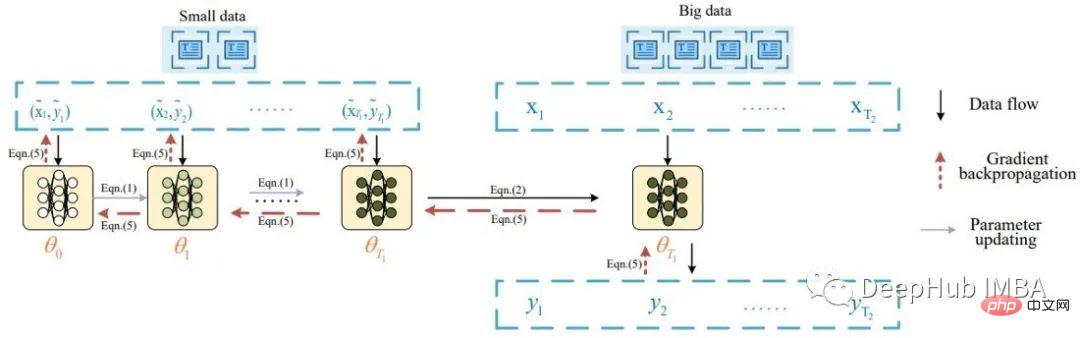
According to the paper, a batch of distilled data is first fed into the model to update its weights. The updated model is then evaluated using real data and the signal is backpropagated to the distilled dataset. The paper reports good classification results (>80% accuracy) on 8 public benchmark datasets.

Following the proposed ideas, I made some minor changes and used a batch of distilled data and multiple real data. The following is the code to create distilled data for intensive retrieval training:

class DistilledData(nn.Module):
def __init__(self, num_labels, M, q_len=64, hidden_size=768):
super().__init__()
self.num_samples = M
self.q_len = q_len
self.num_labels = num_labels
self.data = nn.Parameter(torch.rand(num_labels, M, q_len, hidden_size), requires_grad=True) # i.e. shape: 1000, 4, 64, 768
 
# init using model embedding, xavier, or load from state dict
def init_weights(self, model, path=None):
if model:
self.data.requires_grad = False
print("Init weights using model embedding")
raw_embedding = model.model.get_input_embeddings()
soft_embeds = raw_embedding.weight[:, :].clone().detach()
nums = soft_embeds.size(0)
for i1 in range(self.num_labels):
for i2 in range(self.num_samples):
for i3 in range(self.q_len):
random_idx = random.randint(0, nums-1)
self.data[i1, i2, i3, :] = soft_embeds[random_idx, :]
print(self.data.shape)
self.data.requires_grad = True
 
if not path:
nn.init.xavier_normal_(self.data)
else:
distilled_data.load_state_dict(torch.load(path), strict=False)
 
# function to sample a passage and positive sample as in the article, i am doing dense retrieval
def get_sample(self, label):
q_idx = random.randint(0, self.num_samples-1)
sampled_dist_q = self.data[label, q_idx, :, :]
 
p_idx = random.randint(0, self.num_samples-1)
while q_idx == p_idx:
p_idx = random.randint(0, self.num_samples-1)
sampled_dist_p = self.data[label, p_idx, :, :]
 
return sampled_dist_q, sampled_dist_p, q_idx, p_idx

This is the code to extract the signal onto the distilled data

def distll_train(chunk_size=32):
count, times = 0, 0
print("*********** Started Training *************")
start = time.time()
lap = time.time()
 
for epoch in range(40):
distilled_data.train()
 
for batch in iter(train_dataloader):
count += 1
# get real query, pos, label, distilled data query, distilled data pos, ... from batch
q, p, train_labels, dq, dp, q_indexes, p_indexes = batch
 
for idx in range(0, dq['input_ids'].size(0), chunk_size):
model.train()
 
with torch.enable_grad():
# train on distiled data first
x1 = dq['input_ids'][idx:idx+chunk_size].clone().detach().requires_grad_(True)
x2 = dp['input_ids'][idx:idx+chunk_size].clone().detach().requires_grad_(True)
q_emb = model(inputs_embeds=x1.to("cuda:0"),
attention_mask=dq['attention_mask'][idx:idx+chunk_size].to("cuda:0")).cpu()
p_emb = model(inputs_embeds=x2.to("cuda:0"),
attention_mask=dp['attention_mask'][idx:idx+chunk_size].to("cuda:0"))
loss = default_loss(q_emb.to("cuda:0"), p_emb)
del q_emb, p_emb
 
loss.backward(retain_graph=True, create_graph=False)
state_dict = model.state_dict()
 
# update model weights
with torch.no_grad():
for idx, param in enumerate(model.parameters()):
if param.requires_grad and not param.grad is None:
param.data -= (param.grad*3e-5)
 
# real data
model.eval()
q_embs = []
p_embs = []
for k in range(0, len(q['input_ids']), chunk_size):
with torch.no_grad():
q_emb = model(input_ids=q['input_ids'][k:k+chunk_size].to("cuda:0"),).cpu()
p_emb = model(input_ids=p['input_ids'][k:k+chunk_size].to("cuda:0"),).cpu()
q_embs.append(q_emb)
p_embs.append(p_emb)
q_embs = torch.cat(q_embs, 0)
p_embs = torch.cat(p_embs, 0)
r_loss = default_loss(q_embs.to("cuda:0"), p_embs.to("cuda:0"))
del q_embs, p_embs
 
# distill backward
if count % 2 == 0:
d_grad = torch.autograd.grad(inputs=[x1.to("cuda:0")],#, x2.to("cuda:0")],
outputs=loss,
grad_outputs=r_loss)
indexes = q_indexes
else:
d_grad = torch.autograd.grad(inputs=[x2.to("cuda:0")],
outputs=loss,
grad_outputs=r_loss)
indexes = p_indexes
loss.detach()
r_loss.detach()
 
grads = torch.zeros(distilled_data.data.shape) # lbl, 10, 100, 768
for i, k in enumerate(indexes):
grads[train_labels[i], k, :, :] = grads[train_labels[i], k, :, :].to("cuda:0") 
+ d_grad[0][i, :, :]
distilled_data.data.grad = grads
data_optimizer.step()
data_optimizer.zero_grad(set_to_none=True)
 
model.load_state_dict(state_dict)
model_optimizer.step()
model_optimizer.zero_grad(set_to_none=True)
 
if count % 10 == 0:
print("Count:", count ,"| Data:", round(loss.item(), 4), "| Model:", 
round(r_loss.item(),4), "| Time:", round(time.time() - lap, 4))
# print()
lap = time.time()
 
if count % 100 == 0:
torch.save(model.state_dict(), model_PATH)
torch.save(distilled_data.state_dict(), distill_PATH)
 
if loss < 0.1 and r_loss < 1:
times += 1
 
if times > 100:
print("Training Took:", round(time.time() - start), "seconds")
print("n*********** Training Complete *************")
return
del loss, r_loss, grads, q, p, train_labels, dq, dp, x1, x2, state_dict
 
print("Training Took:", round(time.time() - start), "seconds")
print("n*********** Training Complete *************")

The code such as data loading is omitted here, and the distilled data is trained Finally, we can use it by training a new model on it, for example by training it together with new data.

According to my experiments, a model trained on distilled data (containing only 4 samples per label) achieved the best performance of 66%, while a model trained entirely on raw data also achieved 66% the best performance. The untrained normal model achieved 45% performance. As mentioned above these numbers may not be good for intensive retrieval tasks, but will be much better on categorical data.

For this method to be useful when adjusting the model to fit new data, one needs to be able to extract a much smaller data set than the original data (i.e. ~1%). Refined data can also give you a performance that is slightly lower than or equal to active learning methods.

The advantage of this method is that it can create distilled data for permanent use. The disadvantage is that the extracted data is not interpretable and requires additional training time.

Curriculum/Active training

Curriculum training is a method in which it becomes increasingly difficult to provide training samples to the model during training. When training on new data, this method requires manual labeling of tasks, classifying tasks into easy, medium, or difficult, and then sampling the data. To understand what it means for a model to be easy, medium or hard, I take this picture as an example:

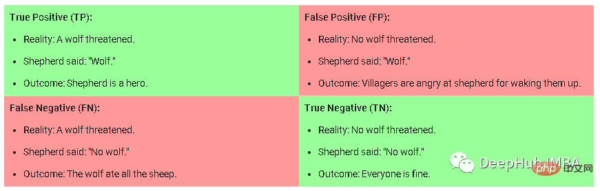
This is the confusion matrix in a classification task, the hard samples are fake Positive (False Positive) refers to a sample that the model predicts is very likely to be True, but is actually not True. Medium samples are those that have a medium to high probability of being correct but are True Negative below the prediction threshold. Simple samples are those with lower likelihood of True Positive/Negative.

Maximally Interfered Retrieval

This is a method introduced by Rahaf in a paper (1908.04742) titled "Online Continual Learning with Maximally Interfered Retrieval". The main idea is that for each new batch of data being trained, if you update the model weights for newer data, you will need to identify the older samples that are most affected in terms of loss values. A limited size memory consisting of old data is retained and the most disturbing samples are retrieved along with each new data batch to train together.

This paper is a well-established paper in the field of continuous learning and has many citations, so it may apply to your case.

Retrieval Augmentation

Retrieval augmentation (Retrieval Augmentation) refers to the technology of augmenting input, samples, etc. by retrieving items from a collection. This is a general concept rather than a specific technology. Most of the methods we've discussed so far are retrieval-related operations to some extent. Izacard's paper titled Few-shot Learning with Retrieval Augmented Language Models uses smaller models to achieve excellent performance in few-shot learning. Retrieval enhancement is also used in many other situations, such as word generation or answering fact questions.

The most common and simplest way to extend the model is to use additional layers during training, but it is not necessarily effective, so it will not be discussed in detail here. An example here is Lewis's Efficient Few-Shot Learning without Prompts. Using additional layers is often the simplest but tried and tested way to get good performance on old and new data. The main idea is to keep the model weights fixed and train one or several layers on new data with a classification loss.

Summary In this article, I introduced 6 methods you can use when training a model on new data. As always one should experiment and decide which method works best, but it is important to note that there are many methods besides the ones I have above, for example data distillation is an active area in computer vision and you can find a lot about it paper. A final note: for these methods to be valuable, they should achieve good performance on both old and new data.

The above is the detailed content of Summary of six common methods of continuous learning: adapting ML models to new data while maintaining the performance of old data. For more information, please follow other related articles on the PHP Chinese website!