As far as machine learning is concerned, audio itself is a complete field with a wide range of applications, including speech recognition, music classification, sound event detection, etc. Audio classification has traditionally used methods such as spectrogram analysis and hidden Markov models, which have proven effective but also have their limitations. Recently VIT has emerged as a promising alternative for audio tasks, with OpenAI’s Whisper being a good example.

GTZAN dataset is the most commonly used public dataset in music genre recognition (MGR) research. The files were collected in 2000-2001 from a variety of sources, including personal CDs, radios, microphone recordings, and represent sounds under a variety of recording conditions.

This data set consists of subfolders, each subfolder is of a type.

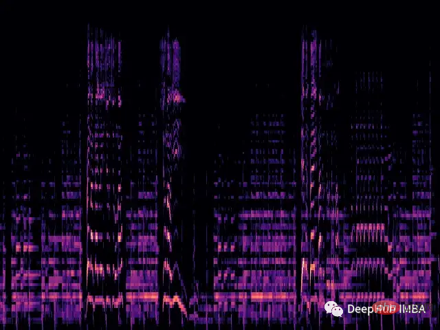
We will load each .wav file and generate the corresponding Mel spectrum through the librosa library.
The mel spectrogram is a visual representation of the spectral content of a sound signal. Its vertical axis represents frequency on the mel scale and the horizontal axis represents time. It is a commonly used representation in audio signal processing, especially in the field of music information retrieval.
Mel scale (English: mel scale) is a scale that takes into account human pitch perception. Because humans do not perceive linear ranges of frequencies, this means we are better at detecting differences at low frequencies than at high frequencies. For example, we can easily tell the difference between 500 Hz and 1000 Hz, but we have a harder time telling the difference between 10,000 Hz and 10,500 Hz, even if the distance between them is the same. So the Mel scale solves this problem, if the differences in the Mel scale are the same, that means the pitch differences perceived by humans will be the same.
def wav2melspec(fp):
 y, sr = librosa.load(fp)
 S = librosa.feature.melspectrogram(y=y, sr=sr, n_mels=128)
 log_S = librosa.amplitude_to_db(S, ref=np.max)
 img = librosa.display.specshow(log_S, sr=sr, x_axis='time', y_axis='mel')
 # get current figure without white border
 img = plt.gcf()
 img.gca().xaxis.set_major_locator(plt.NullLocator())
 img.gca().yaxis.set_major_locator(plt.NullLocator())
 img.subplots_adjust(top = 1, bottom = 0, right = 1, left = 0,
 hspace = 0, wspace = 0)
 img.gca().xaxis.set_major_locator(plt.NullLocator())
 img.gca().yaxis.set_major_locator(plt.NullLocator())
 # to pil image
 img.canvas.draw()
 img = Image.frombytes('RGB', img.canvas.get_width_height(), img.canvas.tostring_rgb())
return imgThe above function will produce a simple mel spectrogram:

Now we load the dataset from the folder and apply the transformation to the image.
class AudioDataset(Dataset):
 def __init__(self, root, transform=None):
 self.root = root
 self.transform = transform
 self.classes = sorted(os.listdir(root))
 self.class_to_idx = {c: i for i, c in enumerate(self.classes)}
 self.samples = []
 for c in self.classes:
 for fp in os.listdir(os.path.join(root, c)):
 self.samples.append((os.path.join(root, c, fp), self.class_to_idx[c]))

 def __len__(self):
 return len(self.samples)

 def __getitem__(self, idx):
 fp, target = self.samples[idx]
 img = Image.open(fp)
 if self.transform:
 img = self.transform(img)
 return img, target

 train_dataset = AudioDataset(root, transform=transforms.Compose([
 transforms.Resize((480, 480)),
 transforms.ToTensor(),
 transforms.Normalize((0.5, 0.5, 0.5), (0.5, 0.5, 0.5))
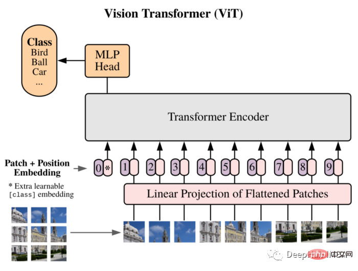
]))We will use ViT as our model: Vision Transformer first introduced an image equal to 16x16 words in the paper, and successfully demonstrated that this method does not Relying on any CNN, a pure Transformer applied directly to the sequence of image patches can perform image classification tasks well.

Split the image into Patches, and use the linear embedding sequence of these Patches as the input of the Transformer. Patches are treated in the same way as tokens (words) in NLP applications.
Due to the lack of inductive bias (such as locality) inherent in CNN, Transformer cannot generalize well when the amount of training data is insufficient. But when trained on large datasets, it does meet or beat the state-of-the-art on multiple image recognition benchmarks.
The implemented structure is as follows:
class ViT(nn.Sequential):
 def __init__(self,
 in_channels: int = 3,
 patch_size: int = 16,
 emb_size: int = 768,
 img_size: int = 356,
 depth: int = 12,
 n_classes: int = 1000,
 **kwargs):
 super().__init__(
 PatchEmbedding(in_channels, patch_size, emb_size, img_size),
 TransformerEncoder(depth, emb_size=emb_size, **kwargs),
 ClassificationHead(emb_size, n_classes)
The training cycle is also a traditional training process:
vit = ViT(
 n_classes = len(train_dataset.classes)
 )

 vit.to(device)

 # train
 train_loader = DataLoader(train_dataset, batch_size=32, shuffle=True)
 optimizer = optim.Adam(vit.parameters(), lr=1e-3)
 scheduler = ReduceLROnPlateau(optimizer, 'max', factor=0.3, patience=3, verbose=True)
 criterion = nn.CrossEntropyLoss()
 num_epochs = 30

 for epoch in range(num_epochs):
 print('Epoch {}/{}'.format(epoch, num_epochs - 1))
 print('-' * 10)

 vit.train()

 running_loss = 0.0
 running_corrects = 0

 for inputs, labels in tqdm.tqdm(train_loader):
 inputs = inputs.to(device)
 labels = labels.to(device)

 optimizer.zero_grad()

 with torch.set_grad_enabled(True):
 outputs = vit(inputs)
 loss = criterion(outputs, labels)

 _, preds = torch.max(outputs, 1)
 loss.backward()
 optimizer.step()

 running_loss += loss.item() * inputs.size(0)
 running_corrects += torch.sum(preds == labels.data)

 epoch_loss = running_loss / len(train_dataset)
 epoch_acc = running_corrects.double() / len(train_dataset)
 scheduler.step(epoch_acc)

print('Loss: {:.4f} Acc: {:.4f}'.format(epoch_loss, epoch_acc))Usage PyTorch trained this custom implementation of the Vision Transformer architecture from scratch. Because the dataset is very small (only 100 samples per class), this affects the performance of the model, and only an accuracy of 0.71 was obtained.
This is just a simple demonstration. If you need to improve the model performance, you can use a larger data set, or slightly adjust the various hyperparameters of the architecture!
The vit code used here comes from:
https://medium.com/artificialis/vit-visiontransformer-a-pytorch-implementation-8d6a1033bdc5
The above is the detailed content of From video to audio: audio classification using VIT. For more information, please follow other related articles on the PHP Chinese website!


