 Technology peripherals
 AI
AI
 Trajectory prediction and planning for autonomous driving under forced merging
Trajectory prediction and planning for autonomous driving under forced merging
Generally speaking, merging is a challenging task for both autonomous and manned driving, especially in dense traffic flow scenarios, because merging vehicles usually need to interact with other vehicles to identify Or create space for safe incorporation. This paper studies the control problem of autonomous vehicles in forced merging scenarios. We propose a new game-based controller called the leader-follower game controller (LFGC).
Among them, a partially considerable leader-follower game model is used to model the interaction between autonomous vehicles and other vehicles with a priori uncertain driving intentions. LFGC estimates the intentions of other vehicles online based on the observed trajectories, predicts their future trajectories, and uses model predictive control (MPC) to plan the self-vehicle trajectory to ensure safety probability while achieving the merge goal. In order to verify the performance of LFGC, we tested it using simulation and NGSIM data, in which LFGC demonstrated an incorporation success rate of up to 97.5%.
01 Introduction
The realization of highly autonomous vehicles still faces many challenges [4]. Completing mandatory merging on the highway is very important. It is a challenging scenario for both manned and autonomous driving. Forced merging usually refers to the scenario where the current lane ends and forced merging is required, such as merging on a highway entrance ramp. In heavy traffic, merging vehicles interact and/or cooperate with vehicles traveling in the target lane.
At this time, the vehicle in the target lane can choose to ignore the merging vehicle (that is, continue driving). At this time, the merging vehicle can only merge behind it; or, in the target lane Vehicles may choose to yield to the merge (i.e., allow the merging vehicle to merge in front of it). To successfully merge into dense traffic flows, autonomous vehicle controllers need to reasonably predict the intention of vehicles in the target lane to continue or yield in order to respond appropriately.
At the same time, the intention of other cars depends not only on the traffic conditions (such as the relative position and speed between the two cars), but also on the driver’s general driving style and personality. , emotions, etc. For example, an aggressive driver may be inclined to keep driving, while a cautious, conservative driver may be inclined to give in. This poses significant challenges to the planning and control of autonomous vehicles.
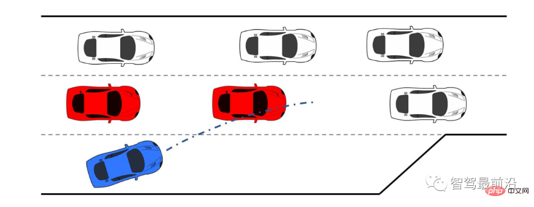
##Figure 1 Blue self-vehicle forced merging scene
Currently, many scholars use the Partially Observable Markov Decision Process (POMDP) framework to deal with the uncertainty of interactions (for example, due to different cooperative intentions of other cars). However, this method has high computational requirements [ 11], which is difficult to use for multi-vehicle interaction.
Reinforcement learning (RL) method is another popular method to set control strategies for lane changing or merging scenarios [12][13]. RL-based methods have the ability to handle complex multi-vehicle interaction scenarios under traffic, but RL lacks interpretability and clear safety guarantees.
In order to achieve more explainable control, some researchers have proposed to add predictive models of vehicle interaction to the control algorithm. For example, [22] uses "Social Generative Adversarial Network (GAN)" to predict the future trajectory of other cars in response to the behavior of the own car. However, SocialGAN does not take into account changes in the driver's style and intention, and requires huge traffic data [23] for training; some studies use game theory methods to model lane changing or merging scenarios [9], [25], Vehicle interactions under [26], [27], [28], [29] can account for different driving styles and/or intentions, such as through game modeling and online estimation of the driver’s cognitive level [26] or [ 30], [31].
In this paper, a new advanced control algorithm is proposed, called the leader-follower game controller (LFGC), for autonomous vehicles in forced merging scenarios. planning and control. In LFGC, explicit game theory is used to model the driver's interaction intention (continue or yield) and the resulting vehicle behavior.
Because the model has multiple parallel leader-follower pairs, it is called a leader-follower game [32]. Considering the uncertainty of interaction, the a priori uncertain leader-follower relationship between two vehicles is modeled as a latent variable. LFGC estimates the leader-follower relationship online based on the observed trajectories and uses a model predictive control (MPC)-based strategy to make optimal decisions for the autonomous vehicle.
Therefore, the proposed LFGC is adapted to evaluate and predict the leader-follower relationship to ensure probabilistic safety while achieving merging.
Compared with existing methods, the contributions and innovations of LFGC are as follows:
1) Use the LFGC game model to predict vehicle trajectories, taking into account The interaction and cooperation intention of other vehicles are connected to MPC control to generate an interpretable control plan.
2) LFGC handles interactions due to different cooperative intentions of other vehicles by modeling uncertainty as a latent variable and Bayesian inference online estimation based on a collection of historical observation trajectories. Uncertainty.
3) LFGC establishes the constraints of vehicle safety requirements (such as collision avoidance) and performs optimization while satisfying clear probabilistic safety characteristics (i.e., within the user-specified safety probability boundary) .
4) LFGC is designed under a continuous state space setting, which reduces the computing cost of discrete space and can handle more complex multi-vehicle interaction scenarios.
5) The feasibility of LFGC has been verified through comprehensive simulation-based case studies, including cases where other vehicles are controlled by various types of driver models, and in NGSIM US Highway 101 Actual cases in the dataset [34]. And in actual case simulations, it shows a success rate of up to 97.5%.
02 Model and control strategy description
In this section, an MPC-based autonomous vehicle is established based on the model representing vehicle and traffic dynamics. Trajectory planning strategies.
Vehicle Dynamics Model
In our use of the kinematic bicycle model [35], the continuum of the bicycle model The time equation is as follows,
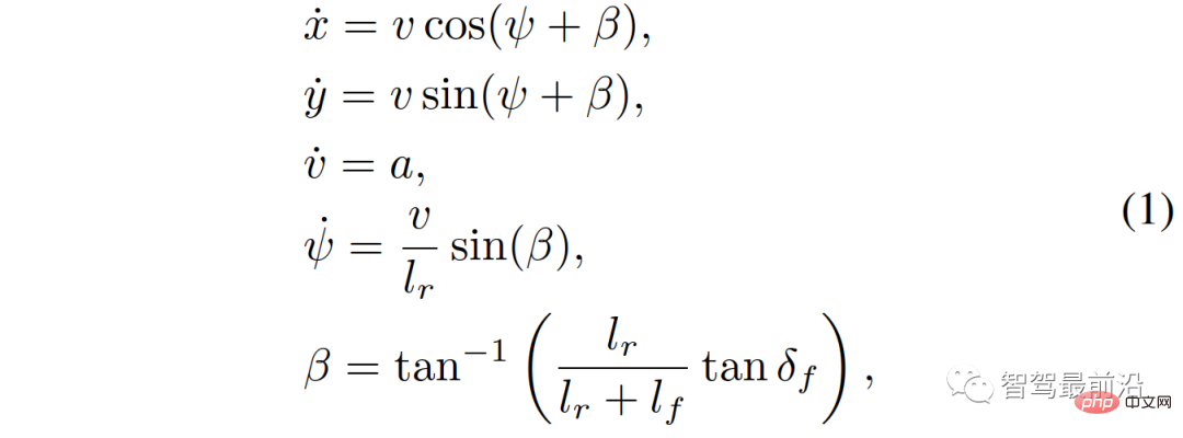
Assume that only the front wheels are steering , no Rear wheel steering (i.e.
  ); x, y are the longitudinal and lateral positions of the vehicle; v is the speed of the vehicle; ψ and β are the yaw angle and slip angle of the vehicle;
  and
and  represent the distance of the vehicle from CG to the front wheel and rear axle; a is the acceleration along the direction of speed v. Control inputs are acceleration and front wheel steering,
  .
.
Dynamic traffic settings
The scenario includes 1 own vehicle and n other vehicles, traffic The states and their dynamics are characterized by the aggregation of states and dynamics of all n 1 vehicles. Specifically, the following discrete time model is used to describe traffic dynamics:

##where, 
represents the traffic status of n 1 vehicles at discrete times, and  represents the set of control inputs of all n 1 vehicles at time t. Each vehicle's status
  includes its xy coordinates, speed and yaw angle; control inputs
reward Function
Reward function  is the mathematical representation of the driver’s driving goal. The traffic state is composed of the states of these two vehicles. , and the reward obtained by the own car depends on the status and control input of the two interacting cars. We consider
 Among them,
  ##,
##,  is a weight vector. Award items
  represent the following common considerations during driving: 1) Safety
  , that is, not colliding with other cars or leaving the road; 2) merging Willingness
  , that is, the distance from the destination lane; 3) Comfort
  , that is, maintaining a reasonable distance from other cars. For a more detailed definition of
  , see [33].
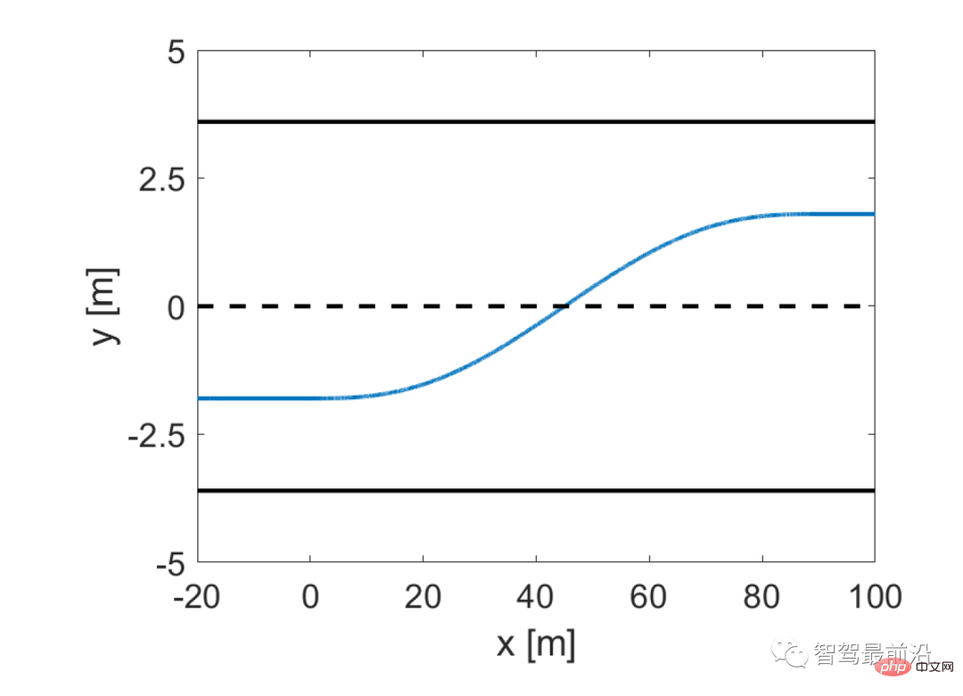
##Figure 2 Lane changing trajectory curve with five degrees of freedom Select trajectories as vehicle motions We consider vehicle motion trajectory samples on  as Action space for each vehicle. Specifically, each trajectory is the time history of the vehicle state
 . According to the vehicle dynamics model (1), the control input time history
 corresponding to each trajectory can be calculated.
For interacting vehicles traveling in the target lane, we only consider their longitudinal motion.
Assuming  and
and  , the kinematic model (1) of these vehicles is simplified to:
At this time, the trajectory starting from the given initial conditions only depends on the acceleration a of [0, T]. At each sample time, 81 acceleration curves are considered, that is, 81 trajectories that satisfy expression (4), thus forming the feasible trajectory range of other vehicles driving in the target lane.
These 81 trajectories comply with the speed constraints .
.
Represent each trajectory as  , m = 1,2,...81, and the set of trajectories is recorded as
The trajectory strategy of the merged vehicle includes lane keeping and lane changing. The lane keeping trajectory generation is similar to (4), and the lane changing trajectory is represented by a fifth-order polynomial. [37]. That is, the solution to the lane changing trajectory requirement can be modeled as the following boundary value problem:
Find the coefficients  and
and  so that the 5th order polynomial
Satisfy the corresponding initial value conditions and final value conditions. The variable ζ in (5) represents continuous time, and ζ=0 for the current sample.
It is also assumed that 1) the vehicle can start changing lanes at any sample time within the planning range, 2) the time required for a complete lane change is constant [37]. Allowing the vehicle to terminate the lane change behavior at any time during the lane change process, which represents the driver's "change of mind" when the previously planned lane change becomes unfeasible/safe. The trajectory after aborting the lane change is generated in a manner similar to the lane change trajectory.
Finally, the trajectories of lane keeping, lane changing and abandonment of lane change are spliced and combined into 162 trajectories, which are used as the feasible region of the strategy.
The extracted trajectory features are: 1) whether/when to start changing lanes; 2) whether/when to stop an inappropriate lane change.
Figure 3 shows the trajectory sampling set when the vehicle does not start to change lanes and when the vehicle is in the process of changing lanes. Denote each trajectory as,m = 1,2,...,162; the trajectory set is,.
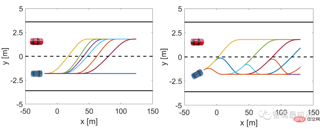
Figure 3 Trajectory sample of the merged vehicle
To sum up the definition A feasible trajectory as a decision output. At the same time, the time history of the control inputs corresponding to these trajectories can be calculated based on the vehicle dynamics model (1). The planned trajectory can be actually transferred to the underlying vehicle motion controller.
Model Predictive Control Strategy
#Consider an MPC-based autonomous vehicle trajectory planning strategy, considering the signal Existence of interactive vehicles: At each sample time t, the self-vehicle calculates an optimal trajectory, 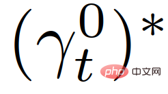 , based on maximizing its cumulative reward within the planning range:

Among them,  represents the predicted traffic status at discrete time t τ, and
  and
and 
represent the predicted control inputs of the own vehicle and the interactive vehicle at t τ, respectively. The parameter λ∈(0,1) is the profit and loss coefficient of future rewards, that is, priority is given to current rewards. In (6), 
represents the reward of the self-vehicle at t τ, as described in Section II-C.  represents a set of safety values for traffic states, used to enforce strict safety regulations. (Such as anti-collision, road boundary constraints, etc.). After obtaining the optimal trajectory
 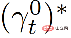 , the vehicle uses the control input
 corresponding to the trajectory to update its status within a sampling period, and then in the next Repeat the above steps for a sampling time instant t1.
03 Game theory model of vehicle cooperative behavior and explicit representation using imitation learning
This section introduces The leader-follower game model used in this article. In order to simplify the online calculation of the game theory model, imitation learning is used to obtain an explicit model based on neural networks to online predict the trajectory of the interactive vehicle's response to merge into the self-vehicle behavior in the MPC-based overall trajectory planning strategy.
Leader-Follower Game Theory Model
In this paper, we consider pair-based leadership A parametric theoretical model of leader-follower interaction is used to represent the driver's cooperative intention and the resulting vehicle behavior, which is called the leader-follower game model. In this model, the vehicle (or driver) that decides to proceed ahead of the other vehicle is the leader of the pair, while the vehicle that decides to yield to the other vehicle is the follower of the pair. Leaders and followers use different decision-making strategies. This leader-follower game theory model was originally proposed in [32]. This game theory model is briefly reviewed here to introduce its application in the forced highway merge scenario.
indicates that the trajectories of the leader and the follower are and respectively, where the sum is the feasible trajectory set of the leader and the follower. Assume that both parties in the game have made the decision to maximize their cumulative rewards, respectively recorded as and , defined as follows:

which represents the role in the game , is the reward function of the leader/follower, and represents the control input corresponding to the sum of their trajectories.
Specifically, we model the interactive decision-making process of leaders and followers as follows:

where  (different from
  ) is the optimal trajectory of the leader (different from the follower), depending on the current traffic state,
  and
and  are defined as follows:

in

 .
.
Decision model (8)-(11) in forced merging can be explained as: a follower represents a driver who intends to give in. Due to uncertainty about the actions of other drivers, followers decide to take an action that maximizes their worst-case reward via (9) and (11), assuming that other drivers are free to act. A leader represents a driver who intends to keep going, assuming the other driver will give in. Therefore, the leader uses the follower model to predict another driver's action and, via (8) and (10), maximizes the leader's own reward given the predicted follower's action. This leader-follower game model is partly derived from the Stackelberg game model [38], but relaxes some assumptions that do not apply to driver interactions. Reference can be made to [32] for a more detailed understanding of the leader-follower game model and its effectiveness in modeling driver interactions in multi-vehicle scenarios.
Please note that this model does not imply that a leader vehicle always forces merging vehicles to merge behind it or that a follower vehicle always forces merging vehicles to merge in front of it. , in the following two examples, the merging vehicle may merge in front of the leader vehicle: 1) The merging vehicle is in front of the leader vehicle, with a large enough distance to allow safe merging. 2) The merging vehicle is about to reach the end of its lane. Because leaving the road results in a large penalty (see Section 2-c), as long as the merging of the self-vehicle does not cause a collision (the penalty of collision is greater than leaving the road), the self-vehicle can choose to merge before the oncoming vehicle to avoid a large collision. punishment,.
The above shows that in our decision-making model (8)-(11), the role of leader-follower is not assigned by the spatial position of the vehicle (the leader is not necessarily is the vehicle in front). In addition, the model allows the self-vehicle to force the target lane traffic flow to merge: as the self-vehicle approaches the target lane, it will increasingly prefer to merge to avoid being penalized for leaving the road. At this time, the self-vehicle will be in the target lane. They are all leaders or they still take the merging action when the current merging gap is not large enough and the merging is not comfortable enough. Models (8)-(11) indicate that the leader identity of the interacting vehicle can predict the merging vehicle's subsequent merging motivation. Subsequently, for the sake of their own safety and comfort, the merging vehicles will also slow down and widen the distance between them to ensure merging.
Leaders who explicitly express game strategies through imitation learning
(8)-(11) Ability to drive based on The driver's intention and current traffic status information can be used to predict the decision-making and trajectory of other vehicles, that is, the leader's optimal action strategy and the follower's optimal action strategy can be obtained through (8)-(11). However, repeated online calculations of (8)-(11) will be time-consuming. Therefore, we will use imitation learning to represent and explicitly.
Referring to [39], we use supervised learning (specifically using imitation learning) representation.
Imitation learning is a supervised learning problem, where the agent will learn a strategy by observing the behavior of experts. Experts can be artificial or artificial intelligence agents, and in our work, what is obtained by (8)-(11) is the expert strategy.
We obtained a simulated strategy using the “dataset aggregation” algorithm [40].
Among them, the overall learning goal of the data set aggregation algorithm can be described as:

represents using θ (Neural network weights) parameterized strategy, representing the loss function, see [39] and [40] for details on imitation learning and "data set aggregation" algorithms.
The imitation learning strategy of learning (8)-(11) can predict the decision-making and future development trajectory of his car while understanding the driver's cooperative intention. However, in a given traffic scenario, we may not know the cooperative intentions of other drivers in advance, because the driver's intention depends not only on the traffic situation (e.g., the relative position and speed between the two vehicles) but also on the driver's intention style/genre. We model the uncertainty of other vehicles' cooperative intentions as latent variables, which will be used to estimate the cooperative intentions of other vehicles and use predictive control methods to obtain optimal trajectories in autonomous vehicle planning and control problems.
04 Decision-making under uncertainty of cooperation intention
Below we describe the highway under uncertainty of cooperation intention Forced merger decision algorithm, leader-follower game controller (LFGC). During the forced merging process, we generate an estimate of other drivers' cooperative intentions as described in this section, based on which we model (6) as a pairwise interactive multi-vehicle control strategy.
Estimating the cooperation intention of interacting vehicles
Using the guided follower game, based on the cooperation intention of other vehicle drivers Behavior modeling with intent. Vehicles that yield are modeled as followers in the game, and vehicles that continue (without yielding) are modeled as leaders. That is, the cooperative intention of the interactive vehicle can be estimated by estimating its role in the leader-follower game.
To achieve this, we consider the traffic dynamics model (2) and the optimal actions of the leader or follower (8) and (9). From the perspective of the self-vehicle, the interactive vehicle is playing a leader-follower game, and the dynamic traffic model can be written as

##Where  is the control of the own vehicle,
  is the control of the interactive vehicle, which is obtained by the leader-follower game,
  {leader, follower} represents the follower or leader, and
  is the first control input, corresponding to
 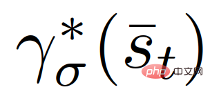 in (8) (9) the optimal trajectory. Now the only input to (14) is the control of the own vehicle
 .
.
Considering that in reality, the decision-making of other cars does not necessarily follow the optimal strategy calculated from (8) and (9), so Gaussian noise is added, assuming The system works according to (14):

where is the additive Gaussian noise with a mean and covariance of 0.
Assume that the self-car has a prior belief about σ, expressed as, where {leader, follower}. Then based on all previous traffic states and all actions taken by the self-vehicle
The self-vehicle needs to calculate or maintain a posteriori belief about the leader or follower role of the interactive vehicle,  .
.
Using the hybrid estimation algorithm proposed in [41], the conditional posterior belief of the leader or follower role of the interactive vehicle can be calculated.
Specifically, identifying the leader or follower role of an interactive vehicle can be expressed as:

 is the conditional probability;
  is the role of the role of the car from
  to ## The transition probability of
  #;
#;  is the likelihood function of the acting car role
  , defined as:

In the formula,  is the probability density function of the normal distribution, the mean is 0, and the coherence The variance W is evaluated at
  ;
; 
is the normalization constant.
Assume that the role of the interacting vehicle remains unchanged during the merge, i.e. when 
 , when
, the posterior belief of the leader or follower role of the interactive vehicle can be updated using the following equation:

where  is the prior belief in the role of the leader or follower of the interactive vehicle.
Control strategy for multi-vehicle interaction
When traffic is heavy, there may be Multiple vehicles interfere with the merging of your own vehicle, as shown in Figure 1. A low-complexity solution is for the self-vehicle to only consider interactions with the first vehicle, and then start interacting with the second vehicle after the first vehicle moves away. However, this may lead to a delay in estimating the intentions of the following vehicle, causing the own vehicle to lose the opportunity to merge.
Another solution is to interact with multiple vehicles at the same time. At this time, a model needs to be built to predict the behavior of the interactive vehicle. Although the 2-player leader-follower game described in Section 3 can be extended to a multi-player leader-follower game by considering multi-level decision-making hierarchies, the model complexity will grow exponentially as the number of players increases. When there are more than 3 players, it is difficult to obtain Stackelberg equilibrium [42]. Therefore, we propose a computationally tractable method to extend the framework to multi-vehicle interactions by considering pairwise interactions.
When there are m interacting vehicles, we consider the pairwise interaction between the self-vehicle and each interacting vehicle, and then construct m vehicles containing the self-car and the kth other The traffic state of the vehicle state is expressed as , and the dynamic model of each is given by the following formula:

Similarly, we can use  {leader, follower} to represent the paired leader or follower role of the k-th interactive vehicle, represented by
  The set of all previous paired traffic states and actions of the self-vehicle, i.e.,

then We can utilize (19) to update the beliefs of each interacting vehicle’s leader or follower role,  ,
, 
{leader ,follower}. The MPC-based control strategy in (6) can be restated as:
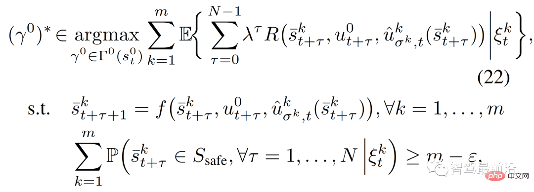
where, 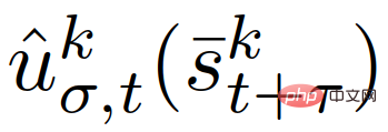 is the first control input corresponding to the trajectory of the training strategy
  in (12), and ε∈[0,1] represents the (user-specified) required Constraints satisfy probability levels.
The expectation in the objective function can be solved according to (23);

##where 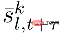 is the role of the given interactive vehicle
  ’s predicted traffic status, and the last constraint in (22) can be passed,

Among them,  is the indicator function of b in set B. Note that the last constraint in (22) enforces the following condition,

which means that any pairwise interaction enters an unsafe state (e.g. , the probability of collision and leaving the road boundary) is less than ε.
To derive (26), we first represent the events 
 and then

Then applying the last constraint in (22), we can get

The main difference between (6) and (22) is:
1) in (6) is unknown, while in (22) ), they are obtained based on the training strategy of imitation learning;
2) Change the maximization of the cumulative reward in (6) to the maximization of the expected cumulative reward in (22) , to account for probabilistic beliefs in the leader/follower role of interacting vehicles;
3) The expected cumulative reward is changed to the sum of the expected rewards of all pairwise interactions to account for multiple vehicles Uncertain behavior (easy to calculate);
4) The hard constraint becomes a probability constraint, with ε∈[0,1] as the parameter.
The decision-making algorithm proceeds as follows: at sampling time t, the self-vehicle measures the current status of each interactive pair and adds them to the observation vector together with the previous control inputs middle. The beliefs about the leader or follower role of each vehicle are updated according to (19). Then, using the MPC-based control strategy (22), the optimal trajectory
  is obtained by searching all trajectories introduced in Section 2-D, and the self-vehicle applies the first Control the input to update its state. The entire process will be repeated the next time the sample is taken.
It should be noted that the control strategy (22) is "interaction-aware" for the following reasons:
1) It Based on the leader-follower game theory model (8)-(11), predict the trajectory of other cars under different interaction intentions.
#2) These predictions are closed-loop. Specifically, corresponding to the different trajectory planning  of the own vehicle, the trajectory predictions of other vehicles with specific intentions are also different. This situation is because the predicted behavior of other vehicles depends on the traffic state, and the predicted traffic state depends on the planned trajectory of the own vehicle.
3) The objective function in (22) is a conditional expectation, and the constraint indicating safety is a conditional probability, both of which are based on other cars’ intentions (i.e. leader or follower)’s latest estimate,  . At the same time, the other car’s intention is estimated based on his previous interaction behavior.
05 Simulation and Verification Results
In this section, we will present the Leader-Following Game Controller (LFGC ) is applied to the verification results of the forced merging problem of autonomous vehicles. We specifically consider three simulation verifications in which LFGC assumes that the interacting vehicle plays a leader-follower game with the self-vehicle and estimates their leader/follower roles in the game. We also assume that once entering a forced lane change situation, the self-vehicle uses the turn signal to align with the lane, announces its intention to merge, and starts the forced merge process. Therefore, other vehicles interacting with each other will be aware of the own vehicle's intention to merge and respond accordingly.
We first validate LFGC in a leader-follower game using interactive vehicles controlled by either a leader or a follower. We then tested LFGC with interactive vehicles controlled by other types of drivers or real traffic data. Furthermore, we tested the case where an interactive vehicle (IDM) was controlled by an intelligent driver model and the interactive vehicle followed actual US Highway 101 traffic data from the Next Generation Simulation Site [34]. Our simulations were performed on MATLAB R2019a platform on a PC with Intel Xeon E3-1246 v3 @ 3.50 GHz CPU and 16 GB memory.
Leader-Follower Model Interaction Vehicle
First we simulate and control the interaction using leader/follower vehicle, testing LFGC. The scenario we are considering is shown in Figure 4. The autonomous vehicle (blue) in the acceleration lane needs to merge onto the highway before the end of the acceleration lane, while many other vehicles (red, pink, green) are currently on the highway. Driving on the highway. As shown in Figure 4, the self-vehicle starts the forced merging process by deviating towards the lane markings and flashing the turn signal. In this case, the autonomous vehicle needs to interact with other vehicles to achieve a safe merge.

Figure 4 LFGC verification scenario diagram of leader/follower controlling interactive vehicles in the forced highway merge scenario
After testing, Car Ability = Correctly recognizes the intent of the interacting vehicle (i.e. can correctly classify the interacting vehicle as leader/follower)
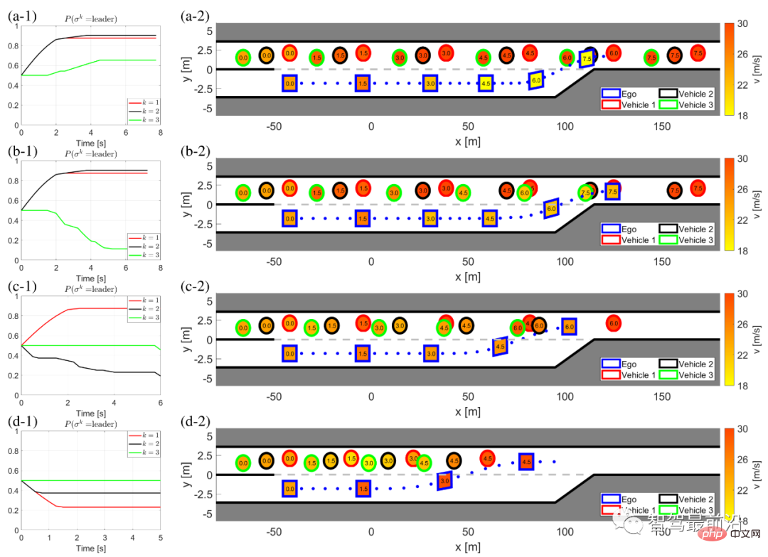
Figure 5 The interaction results of using LFGC with other cars with different combinations of leaders and followers
(a) The other cars have three leaders;
(b) The other car is 1 leader (vehicle 1) and 2 followers (vehicles 2 and 3);
(c ) The other car has two leaders (vehicles 1 and 2) and one follower (vehicle 3);
(d) The other car has three followers.
The left column (a-1) to (d-1) shows the self-car’s belief in the leader of his car in the game. The right columns (a-2) to (d-2) show the time history results of the behavior of the own vehicle and other vehicles during this forced merging process. Specifically, in the right column, the color of the boundary line of each block distinguishes different vehicles, the number in the block represents the time in seconds, the color of each block describes the vehicle speed at that moment, and the blue dotted line represents the self-vehicle traces of. Note that vehicles 1-3 have the same longitudinal position, some longitudinal offset has been added to the figure for better differentiation.
For LFGC, the planning range is N = 4 and the chance constraint parameter is ε = 0.1. Note that a larger N may result in better long-term performance but also longer computation times, whereas a smaller N may emphasize the immediate benefit and thus not be combined in many cases. For the forced highway merges considered in this article, it is generally necessary to choose N such that it exceeds the duration of the lane change (i.e.  ).
).
Figure 5(a) shows the results when the ego car interacts with three leaders. The self-vehicle is able to capture the intention of the interacting vehicles, that is, all vehicles are more likely to become leaders in the game, as shown in Figure 5(a-1). After obtaining this information, the self-vehicle decides to slow down after t = 1 [s] and waits to merge after all interacting vehicles have passed.
When the self-car interacts with a leader (vehicle 1) and two followers (vehicles 2 and 3), the self-car correctly recognizes the intention of the interacting vehicle, as shown in Figure 5 ( b-1) shown. Then after t = 1 [s], the self-vehicle starts to decelerate and successfully merges between vehicle 1 and vehicle 2, as shown in Figure 5(b-2). As shown in Figure 5, (c) is the result of the interaction between the self-vehicle and two leaders (vehicles 1 and 2) and a follower (vehicle 3).
In this case, the ego vehicle observes vehicles 1 and 2 accelerating without yielding, so the ego vehicle decides to slow down and merge between vehicles 2 and 3. We also conducted tests when the self-car interacted with three followers, and the results are shown in Figure 5(d). The self-car observed all intent-generating vehicles, accelerated and merged in front of all interacting vehicles. The average computational time to solve (22) is 0.182 [s] in each time step.
For all cases shown in Figure 5, the initialized beliefs are the same, which means that the self-car does not know in advance whether the interactive vehicle is a leader or a follower. Therefore, the ego vehicle relies on its observations to estimate the leader/follower role of the interaction vector. In the leader-follower game, when all interactive vehicles are controlled by the leader/follower, LFGC can capture the intentions of the interactive vehicles and make corresponding decisions.
His car adopts IDM model type of interaction
The verification results shown in Section 5-A assume that other cars make decisions based on the leader-follower game. LFGC estimates the role of other drivers in the game and makes decisions accordingly. This means that the environment in Section 5-A behaves as expected by LFGC. However, the actual behavior of other drivers may differ from the policy of the leader-follower game. Therefore, we further investigate how the framework responds when other vehicles use an Intelligent Driver Model (IDM).
In this section, use IDM to control other vehicles and interact with your own vehicle. The ego vehicle is still controlled by the LFGC and attempts to estimate the intentions of the interacting vehicles by estimating their corresponding leader or follower roles. IDM is a continuous-time car tracking model, defined by (27) to (29) [43].

##where  is the vertical position;
  is the longitudinal speed;
  is the expected speed of the vehicle;
is the following distance,  is the position of the target vehicle,
  is the length of the target vehicle;
  is the speed difference between the vehicle and the target vehicle;
Based on:  ##
##
Among them,
is the parameter of the IDM model. The physical interpretation of these parameters is the maximum acceleration  , the minimum vehicle following distance

We considered the scenario shown in Figure 6 as a validation test. In Figure 6, all vehicles are preceded by another vehicle (black vehicle 4) traveling at a constant speed. The ego vehicle is still the same as the V-A section and is controlled by the LFGC, which means that from the ego vehicle's perspective, it is playing a leader-follower game with all interacting vehicles. For these three interacting vehicles (Vehicle 1 to 3), they are controlled by IDM, following the preceding vehicle (Vehicle 4) or the own vehicle with a certain time advance t. The IDM model parameters are listed in Table 1. Note that the self-vehicle treats vehicle 4 as the environment vehicle and assumes that it is traveling at a constant speed.

Figure 6 When the other vehicle follows the IDM, the own vehicle uses LFGC to complete the forced merging scene.

Table 1 Intelligent driver model parameters
Fig. 7 shows the results when the own vehicle interacts with other vehicles controlled by IDM with different target vehicles and different desired times.
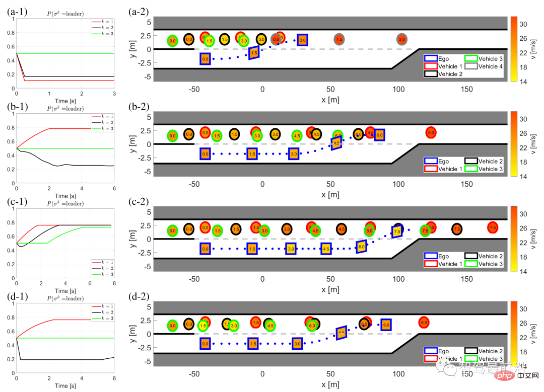
Figure 7: LFGC’s interaction results for other vehicles with different targets and expected times controlled by IDM
(a) Vehicle 1 generates (follows its own vehicle) time progress T = 1 [s], vehicle 2 and vehicle 3 follow T = 0.5 [s];
(b) Vehicle 2 generates (following its own vehicle) T = 0.5 [s], vehicles 1 and 3 follow the previous vehicle T = 0.5 [s];
(c) All vehicles follow the preceding vehicle and T = 0.5 [s]; (d) All vehicles follow the preceding vehicle and T = 1.5 [s].
The left column (a-1) to (d-1) shows the self-car’s belief in the leader of his car in the game. The right columns (a-2) to (d-2) show the time history results of self and other car behavior during this forced merger process. Specifically, in the right column, the color of the boundary line of each block distinguishes different vehicles, the number in the block represents the time in seconds, the color of each block describes the vehicle speed at that moment, and the blue dotted line represents the self-vehicle traces of.
In Figure 7(a), the first interactive vehicle (vehicle 1) intends to yield to its own vehicle, so it chooses to follow its own vehicle that advances for 1 second, and the last two An interactive vehicle follows the preceding vehicle for 0.5 seconds. As can be seen from Figure 7 (a-1), the self-car believes that vehicle 1 has a high probability of becoming a follower in the game, and chooses to merge in front of vehicle 1, as shown in Figure 7 (a-2).
Figure 7(b) shows another situation, that is, the first interactive vehicle (vehicle 1) advances 0.5, and the second interactive vehicle intends to yield to its own vehicle and advances 0.5 Follow your own car. So in this case, from the perspective of the self-vehicle, vehicle 1 has a higher probability of becoming the leader in the game, and vehicle 2 has a higher probability of becoming a follower in the game. Therefore, in this case, the self-vehicle The car merged successfully in front of vehicle 2.
The other two non-yield cases are shown in Figures 7(c) and (d). Figure 7(c) shows the results for all interacting vehicles following the preceding vehicle. From the perspective of the self-vehicle, all interacting vehicles are more likely to become leaders in the game, so the self-car can successfully merge after all vehicles have passed.
In Figure 7(d), all interacting vehicles are moving forward at a speed of 1.5 seconds. In this case, the self-vehicle finds that Vehicle 2 behaves conservatively and believes that Vehicle 2 has a higher probability of becoming a follower in the game. Therefore, the self-vehicle successfully merges between Vehicle 1 and Vehicle 2. The average computational time to solve (22) is 0.198 [s] in each time step.
Other vehicles following real traffic data
We have tested LFGC on leader/follower driven other vehicles and IDM models in leader-follower games. We wanted to further test the performance of the controller using real traffic data. Specifically, we use the US Highway 101 traffic dataset from the Next Generation Simulation (NGSIM) website [34], which is collected by the US Federal Highway Administration and is considered one of the largest publicly available sources of naturalistic driving data. one. The US Highway 101 dataset has been extensively studied in the literature [44], [45], [46].
More specifically, we consider a portion of the US 101 traffic dataset, which contains 30 minutes of vehicle trajectories on the US 101 highway. The time period is from 7:50 to 8:20 in the morning, which represents the congestion before and after the morning rush hour. The dataset contains position and velocity trajectories and vehicle dimensions of approximately 6000 vehicles, with information recorded every 0.1 [s]. An overhead view of the section of US Highway 101 used for data collection is shown in Figure 8. The study segment included the highway's five main lanes, an on-ramp to the highway, an off-ramp off the highway, and an auxiliary lane for merging onto and exiting the highway.
As discussed in [47], the US101 dataset contains a significant amount of noise due to video analysis and numerical differentiation. To overcome this shortcoming, we utilize the Savitsky-Gorey filter [48] to smooth the vehicle's position and update its corresponding velocity. The Savitzky-Golay filter performs well on the US101 dataset with a time window length of 21 [45]. An original vehicle trajectory and the corresponding smoothed vehicle trajectory are shown in Figure 9.
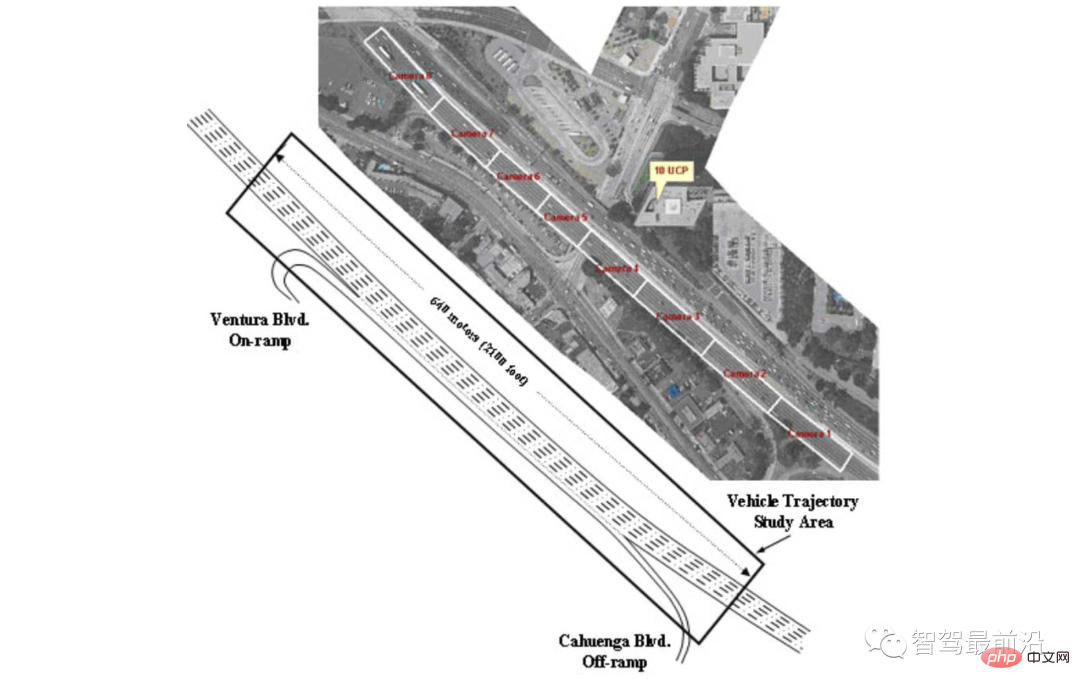
##Figure 8 Overhead view of the highway used to collect US 101 traffic data [34]
This section includes the five main lanes of the highway, an on-ramp to the highway, an exit ramp to exit the highway, and an Auxiliary lanes for merging onto and exiting the motorway.
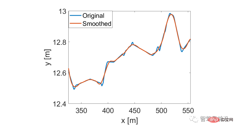
Figure 9 Smoothed from the US 101 traffic data set using Savitsky-Gorey filter Vehicle Trajectories
#For validation testing of LFGC, we focus on on-ramp and auxiliary lanes to identify all merging vehicles. After identifying the merging vehicles and corresponding scenarios, we identify the interacting vehicles according to Figure 10. Specifically, we consider the first vehicle in the target lane within a 2-second period as the first interacting vehicle, and the consecutive vehicles as the second and third vehicles. For all other vehicles present in the scene, the self-vehicle will treat them as environmental vehicles and assume that they are traveling at a constant speed. An identified merge scenario is shown in Figure 11.

Figure 10 Selection of interactive vehicles: own vehicle (blue vehicle) with selection box (red box ) are interactive vehicles
#The front end of the selection box progresses 2 times before the own car. The first vehicle on the target lane in the selection box is the first interactive vehicle, and the following vehicles are the second and third interactive vehicles. For all other vehicles on the highway, they are treated as ambient vehicles and assumed to maintain a constant speed.
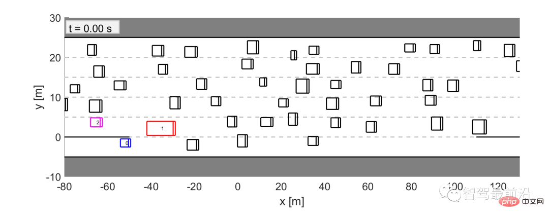
##Figure 11 A merged scenario determined from the US 101 traffic data set In this scenario, vehicle 0 (blue vehicle) is the merged vehicle, and we let LFGC control vehicle 0. According to our criteria for selecting interactive vehicles, vehicle 1 (red vehicle) and vehicle 2 (pink vehicle) are selected as interactive vehicles, and all other vehicles (black vehicles) are regarded as environmental vehicles, assuming that they drive at a fixed speed. For each merged scenario, instead of letting the self-vehicle track traffic data, we use LFGC to control the self-vehicle’s behavior and resulting trajectory. For all other vehicles, including interacting vehicles and environmental vehicles, they follow the corresponding trajectories as they appear in the US 101 traffic dataset. The LFGC then needs to estimate the intentions of the interacting vehicles and control the self-vehicle to merge appropriately. Note that during data collection, interacting and ambient vehicles may interact with merging vehicles during actual traffic. Since 1) the LFGC may act differently from human operation, the behavior of the interactive vehicle or environmental vehicle does not respond to the behavior of the self-vehicle. Instead, their behavior is predetermined by the traffic data set, so conservative measures need to be taken to avoid collisions; 2) Traffic is dense, leaving no safe margin for self-vehicles to merge without intersecting the collision boxes of other vehicles. 
Table 2: Verification of LFGC statistics using US101 traffic data set
"Success" means that the self-vehicle successfully merged into the target lane without any collision. "Failed to merge" means that the own vehicle cannot merge at the end of the auxiliary lane. "Collision" refers to a collision between your own vehicle and another vehicle. Finally, the author took a screenshot of the merging process for analysis.
In Figure 12, we show a screenshot of a successful merge. In these figures, the blue vehicle is controlled by LFGC, and the gray box represents the actual position of the self-vehicle in the data set. All other vehicles (including red interactive vehicles and black environmental vehicles) follow their corresponding trajectories in the dataset. The self-vehicle controlled by the LFGC makes similar decisions to the human driver (gray box): both the LFGC and the human driver first try to accelerate and merge in front of the truck (vehicle 1). However, upon realizing that the truck was more likely to continue to yield, the self-vehicle decided to slow down and merge behind the truck.
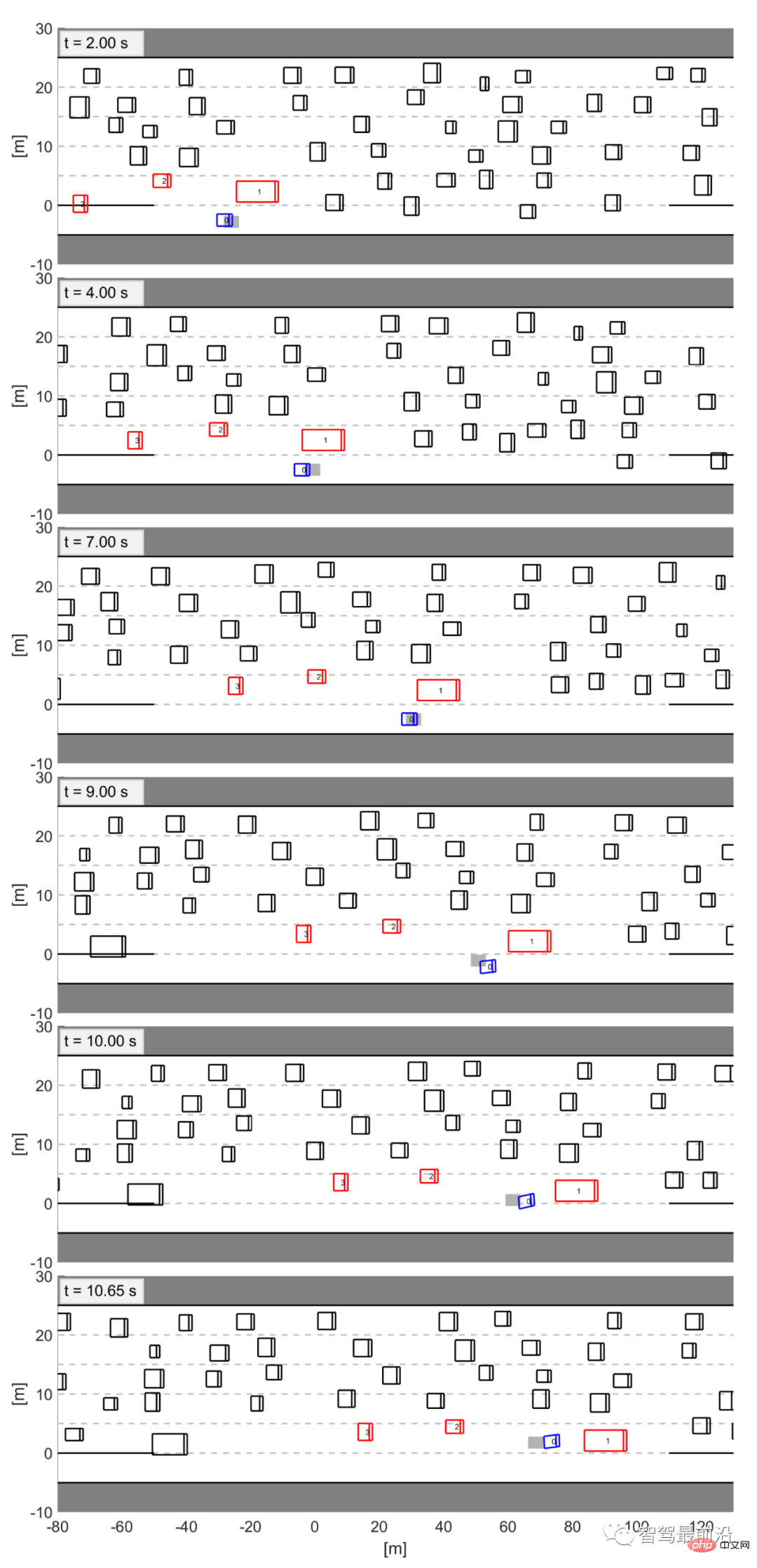
Figure 12 Illustration of a successful merge when validating LFGC on the US Highway 101 dataset
The blue vehicle is the self-vehicle controlled by LFGC, and the gray box is the location of the self-vehicle appearing in the data.
06 Conclusion
In this paper, we proposed a framework for autonomous vehicle planning and control in merged scenarios. Follower Game Controller (LFGC). LFGC takes the interaction uncertainty caused by different driver intentions as a latent variable, estimates other driver intentions, and selects actions to promote self-vehicle merging. In particular, LFGC is able to implement an explicit probabilistic safety property, that is, subject to vehicle safety constraints.
By considering the pairwise interaction between the self-vehicle and the interacting vehicle, LFGC is able to handle interactions with multiple vehicles in a computable way. Finally, multiple simulation-based verifications are conducted to demonstrate the effectiveness of LFGC, including scenarios where other cars follow the leader or follower in the game, an intelligent driver model (IDM), and actual US Highway 101 data.
This article is translated from
"Interaction-Aware Trajectory Prediction and Planning for Autonomous Vehicles in Forced Merge Scenarios》
The above is the detailed content of Trajectory prediction and planning for autonomous driving under forced merging. For more information, please follow other related articles on the PHP Chinese website!

Hot AI Tools

Undresser.AI Undress
AI-powered app for creating realistic nude photos

AI Clothes Remover
Online AI tool for removing clothes from photos.

Undress AI Tool
Undress images for free

Clothoff.io
AI clothes remover

Video Face Swap
Swap faces in any video effortlessly with our completely free AI face swap tool!

Hot Article

Hot Tools

Notepad++7.3.1
Easy-to-use and free code editor

SublimeText3 Chinese version
Chinese version, very easy to use

Zend Studio 13.0.1
Powerful PHP integrated development environment

Dreamweaver CS6
Visual web development tools

SublimeText3 Mac version
God-level code editing software (SublimeText3)

Hot Topics
 Why is Gaussian Splatting so popular in autonomous driving that NeRF is starting to be abandoned?
Jan 17, 2024 pm 02:57 PM
Written above & the author’s personal understanding Three-dimensional Gaussiansplatting (3DGS) is a transformative technology that has emerged in the fields of explicit radiation fields and computer graphics in recent years. This innovative method is characterized by the use of millions of 3D Gaussians, which is very different from the neural radiation field (NeRF) method, which mainly uses an implicit coordinate-based model to map spatial coordinates to pixel values. With its explicit scene representation and differentiable rendering algorithms, 3DGS not only guarantees real-time rendering capabilities, but also introduces an unprecedented level of control and scene editing. This positions 3DGS as a potential game-changer for next-generation 3D reconstruction and representation. To this end, we provide a systematic overview of the latest developments and concerns in the field of 3DGS for the first time.
 How to solve the long tail problem in autonomous driving scenarios?
Jun 02, 2024 pm 02:44 PM
Yesterday during the interview, I was asked whether I had done any long-tail related questions, so I thought I would give a brief summary. The long-tail problem of autonomous driving refers to edge cases in autonomous vehicles, that is, possible scenarios with a low probability of occurrence. The perceived long-tail problem is one of the main reasons currently limiting the operational design domain of single-vehicle intelligent autonomous vehicles. The underlying architecture and most technical issues of autonomous driving have been solved, and the remaining 5% of long-tail problems have gradually become the key to restricting the development of autonomous driving. These problems include a variety of fragmented scenarios, extreme situations, and unpredictable human behavior. The "long tail" of edge scenarios in autonomous driving refers to edge cases in autonomous vehicles (AVs). Edge cases are possible scenarios with a low probability of occurrence. these rare events
 Choose camera or lidar? A recent review on achieving robust 3D object detection
Jan 26, 2024 am 11:18 AM
0.Written in front&& Personal understanding that autonomous driving systems rely on advanced perception, decision-making and control technologies, by using various sensors (such as cameras, lidar, radar, etc.) to perceive the surrounding environment, and using algorithms and models for real-time analysis and decision-making. This enables vehicles to recognize road signs, detect and track other vehicles, predict pedestrian behavior, etc., thereby safely operating and adapting to complex traffic environments. This technology is currently attracting widespread attention and is considered an important development area in the future of transportation. one. But what makes autonomous driving difficult is figuring out how to make the car understand what's going on around it. This requires that the three-dimensional object detection algorithm in the autonomous driving system can accurately perceive and describe objects in the surrounding environment, including their locations,
 Have you really mastered coordinate system conversion? Multi-sensor issues that are inseparable from autonomous driving
Oct 12, 2023 am 11:21 AM
The first pilot and key article mainly introduces several commonly used coordinate systems in autonomous driving technology, and how to complete the correlation and conversion between them, and finally build a unified environment model. The focus here is to understand the conversion from vehicle to camera rigid body (external parameters), camera to image conversion (internal parameters), and image to pixel unit conversion. The conversion from 3D to 2D will have corresponding distortion, translation, etc. Key points: The vehicle coordinate system and the camera body coordinate system need to be rewritten: the plane coordinate system and the pixel coordinate system. Difficulty: image distortion must be considered. Both de-distortion and distortion addition are compensated on the image plane. 2. Introduction There are four vision systems in total. Coordinate system: pixel plane coordinate system (u, v), image coordinate system (x, y), camera coordinate system () and world coordinate system (). There is a relationship between each coordinate system,
 This article is enough for you to read about autonomous driving and trajectory prediction!
Feb 28, 2024 pm 07:20 PM
Trajectory prediction plays an important role in autonomous driving. Autonomous driving trajectory prediction refers to predicting the future driving trajectory of the vehicle by analyzing various data during the vehicle's driving process. As the core module of autonomous driving, the quality of trajectory prediction is crucial to downstream planning control. The trajectory prediction task has a rich technology stack and requires familiarity with autonomous driving dynamic/static perception, high-precision maps, lane lines, neural network architecture (CNN&GNN&Transformer) skills, etc. It is very difficult to get started! Many fans hope to get started with trajectory prediction as soon as possible and avoid pitfalls. Today I will take stock of some common problems and introductory learning methods for trajectory prediction! Introductory related knowledge 1. Are the preview papers in order? A: Look at the survey first, p
 Let's talk about end-to-end and next-generation autonomous driving systems, as well as some misunderstandings about end-to-end autonomous driving?
Apr 15, 2024 pm 04:13 PM
In the past month, due to some well-known reasons, I have had very intensive exchanges with various teachers and classmates in the industry. An inevitable topic in the exchange is naturally end-to-end and the popular Tesla FSDV12. I would like to take this opportunity to sort out some of my thoughts and opinions at this moment for your reference and discussion. How to define an end-to-end autonomous driving system, and what problems should be expected to be solved end-to-end? According to the most traditional definition, an end-to-end system refers to a system that inputs raw information from sensors and directly outputs variables of concern to the task. For example, in image recognition, CNN can be called end-to-end compared to the traditional feature extractor + classifier method. In autonomous driving tasks, input data from various sensors (camera/LiDAR
 SIMPL: A simple and efficient multi-agent motion prediction benchmark for autonomous driving
Feb 20, 2024 am 11:48 AM
Original title: SIMPL: ASimpleandEfficientMulti-agentMotionPredictionBaselineforAutonomousDriving Paper link: https://arxiv.org/pdf/2402.02519.pdf Code link: https://github.com/HKUST-Aerial-Robotics/SIMPL Author unit: Hong Kong University of Science and Technology DJI Paper idea: This paper proposes a simple and efficient motion prediction baseline (SIMPL) for autonomous vehicles. Compared with traditional agent-cent
 FisheyeDetNet: the first target detection algorithm based on fisheye camera
Apr 26, 2024 am 11:37 AM
Target detection is a relatively mature problem in autonomous driving systems, among which pedestrian detection is one of the earliest algorithms to be deployed. Very comprehensive research has been carried out in most papers. However, distance perception using fisheye cameras for surround view is relatively less studied. Due to large radial distortion, standard bounding box representation is difficult to implement in fisheye cameras. To alleviate the above description, we explore extended bounding box, ellipse, and general polygon designs into polar/angular representations and define an instance segmentation mIOU metric to analyze these representations. The proposed model fisheyeDetNet with polygonal shape outperforms other models and simultaneously achieves 49.5% mAP on the Valeo fisheye camera dataset for autonomous driving


