 Technology peripherals
 AI
AI
 Detailed comparison of generative models VAE, GAN and flow-based models
Detailed comparison of generative models VAE, GAN and flow-based models
Two years after Ian Goodfellow and other researchers introduced generative adversarial networks in a paper, Yann LeCun called adversarial training "the most interesting idea in ML in the past decade." Although GANs are interesting and promising, they are only part of a family of generative models that solve traditional AI problems from a completely different perspective. In this article we will compare three common generative models.
Generation algorithm
When we think of machine learning, the first thing that probably comes to mind is the discriminant algorithm. Discriminative models are the prediction of labels or categories of input data based on its characteristics and are at the heart of all classification and prediction solutions. In contrast to these models, generative algorithms help us tell stories about the data and provide possible explanations of how the data was generated. Unlike discriminative algorithms, which map features to labels, generative models try to predict features given a label.
Distinguish the relationship between the label y and the feature x defined by the model, and generate the model to answer the question "How do you get y". The generative model model is P(Observation/Cause), and then uses Bayes' theorem to calculate P(Cause/Observation). In this way, they can capture p(x|y), the probability of x given y, or the probability of a feature given a label or class. So in fact, generative algorithms can also be used as classifiers, probably because they model the distribution of individual classes.
There are many generative algorithms, but the most popular models that fall into the category of deep generative models are variational autoencoders (VAEs), gans, and flow-based models.
VAE
A variational autoencoder (VAE) is a generative model that "provides a probabilistic description of observations in a latent space." Simply put, this means that VAE stores latent attributes as probability distributions.
The idea of variational autoencoders (Kingma & Welling, 2014) or VAEs is deeply rooted in variational Bayesian and graphical model methods.
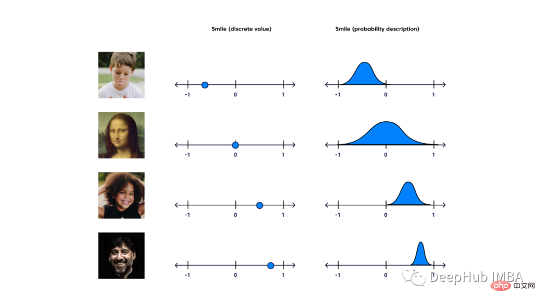
The standard autoencoder consists of 2 similar networks, an encoder and a decoder. The encoder takes the input and converts it into a smaller representation, which the decoder can use to convert it back to the original input. The latent space into which they transform the input and the space in which their encoding vectors lie may not be continuous. This is a problem for generative models, as we all want to sample randomly from a latent space, or generate variations of the input image from a continuous latent space.
The variational autoencoder has a continuous latent space, which makes random sampling and interpolation more convenient. To achieve this, the hidden nodes of the encoder do not output the encoding vector, but instead output two vectors of the same size: a mean vector and a standard deviation vector. Each hidden node considers itself Gaussian distributed. The i-th element of the mean and standard deviation vector here corresponds to the mean and standard deviation value of the i-th random variable. We sample from this distribution vector and the decoder randomly samples from the probability distribution of the input vector. This process is random generation. This means that even for the same input, when the mean and standard deviation are held constant, the actual encoding will differ in each pass.
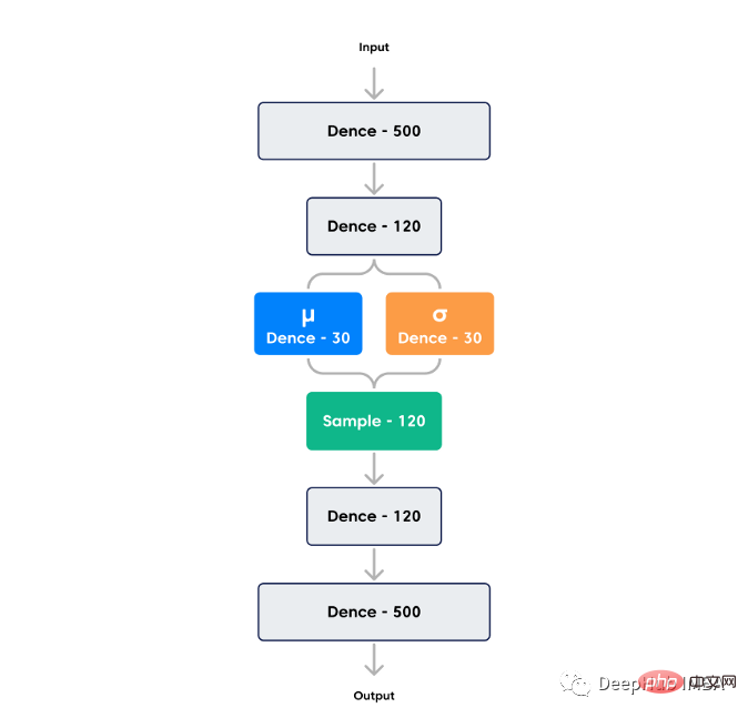
The loss of the autoencoder is to minimize the reconstruction loss (how similar the output is to the input) and the latent loss (how close the hidden nodes are to the normal distribution). The smaller the potential loss, the less information can be encoded, so the reconstruction loss will increase, so there is a trade-off between the potential loss and the reconstruction loss. When the potential loss is small, the generated image will be too similar to the training image, resulting in poor performance. When the reconstruction loss is small, the reconstructed image effect during training is better, but the generated new image is quite different from the reconstructed image, so a good balance needs to be found.
VAEs can handle various types of data, sequential and non-sequential, continuous or discrete, even labeled or unlabeled, which makes them very powerful generation tools.
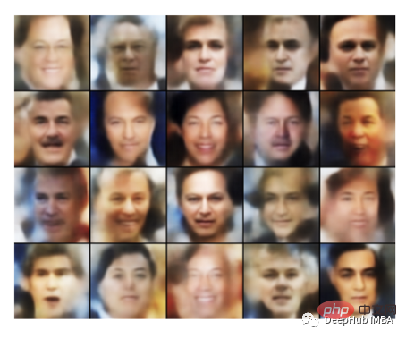
But a major drawback of VAEs is the blurry output they generate. As Dosovitskiy and Brox pointed out, VAE models often produce unrealistic and ambiguous samples. This is caused by the way the data distribution is recovered and the loss function is calculated. A 2017 paper by Zhao et al. suggested modifying VAEs without using variational Bayesian methods to improve output quality.
Generative adversarial networks
Generative adversarial networks (GANs) are a generative model based on deep learning that can generate new content. The GAN architecture was first described in a 2014 paper titled "Generative Adversarial Networks" by Ian Goodfellow et al.
GANs employ a supervised learning approach using two sub-models: a generator model that generates new examples and a discriminator model that attempts to classify examples as real or fake (generated).
Generator: A model used to generate new plausible examples from the problem domain.
Frequency Discriminator: A model used to classify examples as real (from the domain) or fake (generated).
The two models are trained as competitors. Generators produce sample data directly. Its opponent, the discriminator, attempts to distinguish between samples drawn from the training data and samples drawn from the generator. This competitive process continues during training until the discriminator model fails to tell true or false more than half the time, which means that the generator model is generating very realistic data.
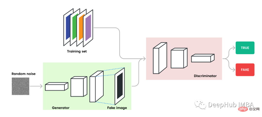
#When the discriminator successfully identifies a real or fake sample, it is rewarded while its parameters remain unchanged. If the generator makes a mistake, it is punished and its parameters are updated. In an ideal world, whenever the discriminator can't tell the difference and predicts "uncertain" (e.g., 50% true or false), the generator can produce a perfect copy from the input domain.
But here each model can overpower the other. If the discriminator is too good, it will return values very close to 0 or 1, and the generator will have trouble getting updated gradients. If the generator is too good, it will exploit the discriminator's weaknesses and cause false negatives. Therefore, the two neural networks must have similar "skill levels" achieved through their respective learning rates. This is also one of the reasons why GAN is difficult to train.
Generator model
The generator takes a fixed-length random vector as input and generates a sample within the defined domain. This vector is randomly drawn from a Gaussian distribution. After training, the points in this multi-dimensional vector space will correspond to the points in the problem domain, forming a compressed representation of the data distribution. This step is similar to VAE. This vector space is called a latent space, or a vector space composed of latent variables. . The GAN's generator will average selected points in the latent space. New points extracted from the latent space can be provided as input to the generator model and used to generate new and different output examples. After training, the generator model is retained and used to generate new samples.
Discriminator model
The discriminator model takes an example as input (either a real sample from the training dataset or generated by a generator model) and predicts a binary class label of real or fake( has been generated). The discriminator is a normal (and easy to understand) classification model.
After the training process, the discriminator is discarded because we are interested in the generator. Of course the discriminator can also be used for other purposes.
GANs can produce feasible samples, but the original GAN also has shortcomings:
- The image is generated by some arbitrary noise. When generating an image with specific characteristics, one cannot be sure what initial noise value will generate that image, but instead needs to search the entire distribution.
- GAN only differentiates between "real" and "fake" images. But there is no constraint that says a photo of a "cat" must look like a "cat." Therefore, it can result in generated images that don't have the actual objects in them, but the styles look similar.
- GANs take a long time to train. A GAN may take several hours on a single GPU and more than a day on a single CPU.
Flow-based models
Flow-based generative models are exact log-likelihood models with tractable sampling and latent variable inference. Flow-based models apply a bunch of reversible transformations to samples from the prior so that the exact log-likelihood of an observation can be calculated. Unlike the previous two algorithms, this model explicitly learns the data distribution, so the loss function is negative log-likelihood.

In nonlinear independent component analysis, the flow model f is constructed as an invertible mapping of high-dimensional random variables x to standard Gaussian latent variables z=f(x) Transform. The key idea in the design of the flow model is that it can be an arbitrary bijective function and can be formed by superposing simple reversible transformations. To summarize: the flow model f is composed of a series of reversible flows as f(x) =f1◦···◦fL(x), with each fi having a tractable inverse and a tractable Jacobian matrix. Mode.
There are two broad categories of flow-based models: models with normalized flow and models with autoregressive flow that attempt to enhance the performance of the base model.
Normalized Flow Model
Being able to perform good density estimation is essential for many machine learning problems. But it is inherently complex: when we need to perform backpropagation in a deep learning model, the embedded probability distribution needs to be simple enough so that the derivatives can be calculated efficiently. The traditional solution is to use Gaussian distributions in latent variable generation models, although most real-world distributions are much more complex. Normalized flow (NF) models, such as RealNVP or Glow, provide a robust approximation of the distribution. They transform a simple distribution into a complex distribution by applying a series of reversible transformation functions. Through a series of transformations, according to the variable transformation theorem, the original variables can be repeatedly replaced with new variables, and finally the probability distribution of the final target variable is obtained.
Model of Autoregressive Flow
When the flow transformation in the normalized flow is framed as an autoregressive model, where each dimension in the vector variable is conditioned on the previous dimension, the flow model This change in is called autoregressive flow. It is a step forward compared to models with standardized processes.
Commonly used autoregressive flow models are PixelCNN for image generation and WaveNet for one-dimensional audio signals. They all consist of a bunch of causal convolutions - convolution operations that take order into account: predictions at a specific timestamp only use data observed in the past. In PixelCNN, causal convolution is performed by a masked kernel. And WaveNet shifts the output through several timestamps into the future time.
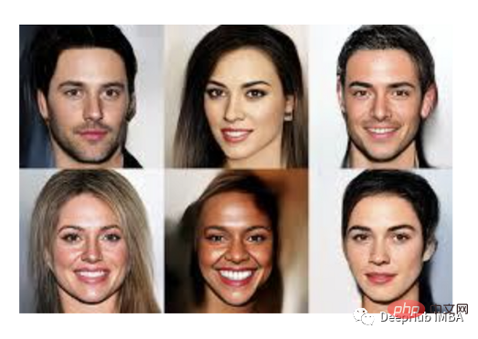
Flow-based models are conceptually very friendly to modeling complex distributions, but they suffer from density estimation performance issues compared to state-of-the-art autoregressive models limits. Although flow models may initially produce good output as an alternative to GANs, there is a significant gap in training computational cost between them, with flow-based models taking several times longer to generate images of the same resolution than GANs.
Summary
Each algorithm has its advantages and limitations in terms of accuracy and efficiency. Although GANs and process-based models generally generate better or closer to real images than VAE, the latter has faster time and better parameter efficiency than process-based models. Here is a comparison summary of the three models:
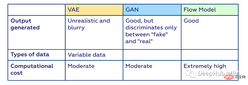
You can see that GAN is very efficient because of its parallelism, but it is not reversible. In contrast, flow models are reversible but not efficient, while vae is reversible and efficient but cannot be computed in parallel. Based on these characteristics, we can make trade-offs between output, training process, and efficiency in actual use.
The above is the detailed content of Detailed comparison of generative models VAE, GAN and flow-based models. For more information, please follow other related articles on the PHP Chinese website!

Hot AI Tools

Undresser.AI Undress
AI-powered app for creating realistic nude photos

AI Clothes Remover
Online AI tool for removing clothes from photos.

Undress AI Tool
Undress images for free

Clothoff.io
AI clothes remover

AI Hentai Generator
Generate AI Hentai for free.

Hot Article

Hot Tools

Notepad++7.3.1
Easy-to-use and free code editor

SublimeText3 Chinese version
Chinese version, very easy to use

Zend Studio 13.0.1
Powerful PHP integrated development environment

Dreamweaver CS6
Visual web development tools

SublimeText3 Mac version
God-level code editing software (SublimeText3)

Hot Topics
 1382
1382
 52
52
 Bytedance Cutting launches SVIP super membership: 499 yuan for continuous annual subscription, providing a variety of AI functions
Jun 28, 2024 am 03:51 AM
This site reported on June 27 that Jianying is a video editing software developed by FaceMeng Technology, a subsidiary of ByteDance. It relies on the Douyin platform and basically produces short video content for users of the platform. It is compatible with iOS, Android, and Windows. , MacOS and other operating systems. Jianying officially announced the upgrade of its membership system and launched a new SVIP, which includes a variety of AI black technologies, such as intelligent translation, intelligent highlighting, intelligent packaging, digital human synthesis, etc. In terms of price, the monthly fee for clipping SVIP is 79 yuan, the annual fee is 599 yuan (note on this site: equivalent to 49.9 yuan per month), the continuous monthly subscription is 59 yuan per month, and the continuous annual subscription is 499 yuan per year (equivalent to 41.6 yuan per month) . In addition, the cut official also stated that in order to improve the user experience, those who have subscribed to the original VIP
 Context-augmented AI coding assistant using Rag and Sem-Rag
Jun 10, 2024 am 11:08 AM
Improve developer productivity, efficiency, and accuracy by incorporating retrieval-enhanced generation and semantic memory into AI coding assistants. Translated from EnhancingAICodingAssistantswithContextUsingRAGandSEM-RAG, author JanakiramMSV. While basic AI programming assistants are naturally helpful, they often fail to provide the most relevant and correct code suggestions because they rely on a general understanding of the software language and the most common patterns of writing software. The code generated by these coding assistants is suitable for solving the problems they are responsible for solving, but often does not conform to the coding standards, conventions and styles of the individual teams. This often results in suggestions that need to be modified or refined in order for the code to be accepted into the application
 Can fine-tuning really allow LLM to learn new things: introducing new knowledge may make the model produce more hallucinations
Jun 11, 2024 pm 03:57 PM
Large Language Models (LLMs) are trained on huge text databases, where they acquire large amounts of real-world knowledge. This knowledge is embedded into their parameters and can then be used when needed. The knowledge of these models is "reified" at the end of training. At the end of pre-training, the model actually stops learning. Align or fine-tune the model to learn how to leverage this knowledge and respond more naturally to user questions. But sometimes model knowledge is not enough, and although the model can access external content through RAG, it is considered beneficial to adapt the model to new domains through fine-tuning. This fine-tuning is performed using input from human annotators or other LLM creations, where the model encounters additional real-world knowledge and integrates it
 Seven Cool GenAI & LLM Technical Interview Questions
Jun 07, 2024 am 10:06 AM
To learn more about AIGC, please visit: 51CTOAI.x Community https://www.51cto.com/aigc/Translator|Jingyan Reviewer|Chonglou is different from the traditional question bank that can be seen everywhere on the Internet. These questions It requires thinking outside the box. Large Language Models (LLMs) are increasingly important in the fields of data science, generative artificial intelligence (GenAI), and artificial intelligence. These complex algorithms enhance human skills and drive efficiency and innovation in many industries, becoming the key for companies to remain competitive. LLM has a wide range of applications. It can be used in fields such as natural language processing, text generation, speech recognition and recommendation systems. By learning from large amounts of data, LLM is able to generate text
 Five schools of machine learning you don't know about
Jun 05, 2024 pm 08:51 PM
Machine learning is an important branch of artificial intelligence that gives computers the ability to learn from data and improve their capabilities without being explicitly programmed. Machine learning has a wide range of applications in various fields, from image recognition and natural language processing to recommendation systems and fraud detection, and it is changing the way we live. There are many different methods and theories in the field of machine learning, among which the five most influential methods are called the "Five Schools of Machine Learning". The five major schools are the symbolic school, the connectionist school, the evolutionary school, the Bayesian school and the analogy school. 1. Symbolism, also known as symbolism, emphasizes the use of symbols for logical reasoning and expression of knowledge. This school of thought believes that learning is a process of reverse deduction, through existing
 To provide a new scientific and complex question answering benchmark and evaluation system for large models, UNSW, Argonne, University of Chicago and other institutions jointly launched the SciQAG framework
Jul 25, 2024 am 06:42 AM
Editor |ScienceAI Question Answering (QA) data set plays a vital role in promoting natural language processing (NLP) research. High-quality QA data sets can not only be used to fine-tune models, but also effectively evaluate the capabilities of large language models (LLM), especially the ability to understand and reason about scientific knowledge. Although there are currently many scientific QA data sets covering medicine, chemistry, biology and other fields, these data sets still have some shortcomings. First, the data form is relatively simple, most of which are multiple-choice questions. They are easy to evaluate, but limit the model's answer selection range and cannot fully test the model's ability to answer scientific questions. In contrast, open-ended Q&A
 SOTA performance, Xiamen multi-modal protein-ligand affinity prediction AI method, combines molecular surface information for the first time
Jul 17, 2024 pm 06:37 PM
Editor | KX In the field of drug research and development, accurately and effectively predicting the binding affinity of proteins and ligands is crucial for drug screening and optimization. However, current studies do not take into account the important role of molecular surface information in protein-ligand interactions. Based on this, researchers from Xiamen University proposed a novel multi-modal feature extraction (MFE) framework, which for the first time combines information on protein surface, 3D structure and sequence, and uses a cross-attention mechanism to compare different modalities. feature alignment. Experimental results demonstrate that this method achieves state-of-the-art performance in predicting protein-ligand binding affinities. Furthermore, ablation studies demonstrate the effectiveness and necessity of protein surface information and multimodal feature alignment within this framework. Related research begins with "S
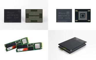 SK Hynix will display new AI-related products on August 6: 12-layer HBM3E, 321-high NAND, etc.
Aug 01, 2024 pm 09:40 PM
According to news from this site on August 1, SK Hynix released a blog post today (August 1), announcing that it will attend the Global Semiconductor Memory Summit FMS2024 to be held in Santa Clara, California, USA from August 6 to 8, showcasing many new technologies. generation product. Introduction to the Future Memory and Storage Summit (FutureMemoryandStorage), formerly the Flash Memory Summit (FlashMemorySummit) mainly for NAND suppliers, in the context of increasing attention to artificial intelligence technology, this year was renamed the Future Memory and Storage Summit (FutureMemoryandStorage) to invite DRAM and storage vendors and many more players. New product SK hynix launched last year


