How to fine-tune very large models with limited GPU resources

Question: What should I do if the model size exceeds the GPU capacity?
#This article is inspired by the "Efficient Deep Learning System" course taught by Yandex Data Analysis Institute.
Preliminary knowledge: It is assumed that the reader already understands the working principles of forward pass and backward pass of neural network. This is crucial to understanding the content of this article. This article uses PyTorch as the framework.
let's start!
When trying to use a large model (aka gpt-2-xl) with over 500 million parameters and your GPU resources are limited and you cannot convert it What should I do if it is installed to run on the GPU, or the batch size defined in the paper cannot be achieved during model training? Maybe you can give up and use a lighter version of the model, or reduce the training batch size, so that you won't get the training results described in the paper.
#However, there are some techniques that can help solve the above problems.
# Let’s discuss some methods on how to fine-tune the GPT-2-XL model with 1.5 billion parameters.
The core of the problem
First, let’s understand the GPU memory problem required to load the model into the GPU. substance.
Assuming that the model has FP32 (32-bit floating point) parameters, this model needs to be trained on the GPU, for example, running the Adam optimizer.
#Through calculation, the results are shocking.
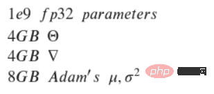
Assume you already have an NVIDIA computer with 12 GB of memory GeForce RTX 3060. First, 1e9 FP32 parameters takes up approximately 4 GB of GPU memory.
#Similarly, the same amount of memory will be reserved for gradients. Therefore, a total of 8 GB of memory has been reserved. Since training has not yet started and the optimizer has not been loaded, loading the optimizer also requires a certain amount of memory. The Adam optimizer needs to store the first and second backups for each parameter, which requires 8 GB of additional memory. Calculating this, you must have approximately 16 GB of GPU memory to correctly load the model onto the GPU. In this example, the GPU only has 12 GB of free memory. Looks bad, right?
However, there are some ways to try to solve this problem, here are the relevant ones:
- Gradient accumulation/micro-batching;
- Gradient checkpoint;
- Model parallel training;
- Pipeline job;
- Tensor parallelization
- Mixed precision training;
- Memory offloading;
- Optimizer 8-bit quantization.
Next, these technologies will be explained in detail.
start

Question: What should I do if the model is larger than the GPU capacity?
- Simple mode: Unable to adapt batch size 1
- Professional mode: parameters cannot be adapted
Overview
If the model is larger than the GPU capacity, even setting the batch size to 1 is not enough, what should I do? There is a solution, which is to set gradient checkpoints. Let’s take a look at this concept. For a simple feedforward neural network containing n layers, the gradient calculation diagram is as follows:

The activation of the neural network layer corresponds to the node marked with f, and during the forward pass, all these nodes are calculated in sequence. The loss gradients corresponding to the activations and parameters of these layers are represented by nodes labeled b. During the backward pass, all these nodes are evaluated in reverse order. The calculation results of f nodes are used to calculate b nodes, so all f nodes are kept in memory after passing forward. Only when backpropagation has progressed far enough to calculate all dependencies of node f, it can be erased from memory. This means: the memory required for simple backpropagation grows linearly with the number of neural network layers n.
The following is the calculation order of these nodes. The purple shaded circle indicates which node needs to be saved to memory at a given time.

##Gradient Checkpoint
Simple backpropagation as described above is computationally optimal: it only computes each node once. However, if you recompute the nodes, you may save a lot of memory. For example, each node can simply be recalculated. The order of execution and the memory used are as shown in the figure below:

This strategy is optimal in terms of memory. However, note that the number of node calculations is scaled n² times, compared to the previous scaling factor of n: each n node is recalculated sequentially n times. Due to the slow computational speed, this method is not suitable for deep learning.
In order to strike a balance between memory and computation, a strategy needs to be proposed that allows nodes to be recalculated, but not too frequently. A strategy used here is to mark a subset of neural network activations as checkpoint nodes.

In this example, choose to mark the sqrt(n)th node as a checkpoint. This way, the number of checkpoint nodes and the number of nodes between checkpoints is between sqrt(n), which means: the amount of memory required also scales in the order of n. The extra computation required by this strategy is equivalent to the computation required by a single forward pass through the network.
Routine:
After learning the details of gradient checkpoints, come See how to apply this concept in PyTorch, it doesn’t look too difficult:
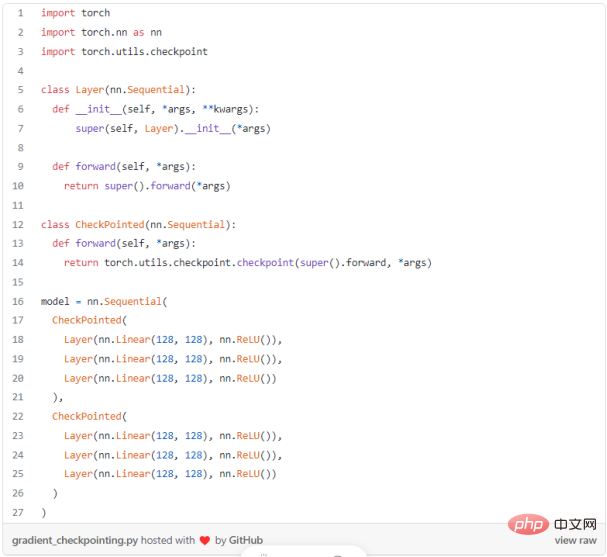
Gradient accumulation/micro-batching

##Overview
Deep learning models are getting larger and larger, and it is difficult to install such large neural networks in GPU memory. Therefore, you are forced to choose a smaller batch size during training, which may lead to slower convergence and lower accuracy.
What is gradient accumulation?
When training a neural network, the data is usually divided into batches, and the neural network predicts the batch labels, which are used to calculate the loss relative to the actual target. Next, perform a backward pass to calculate the gradient and update the model weights. Gradient accumulation modifies the last step of the training process: before continuing to the next mini-batch, save the gradient value and add the new gradient to the previously saved gradient, instead of updating the network weights for each mini-batch . The weights are updated only after the model has processed several mini-batches. Gradient accumulation simulates a larger batch size. If you want to use 64 images in a small batch, if the batch size exceeds 8, a "CUDA memory error..." will be reported. In this case, you can use 8 batches of images and update the weights once after the model processes 64/8 = 8 batches. If you accumulate each gradient from these 8 batches, the results will be (almost) the same, and training can be performed!
Routine:
The standard training loop without gradient accumulation is usually:
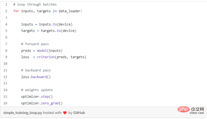
In PyTorch, gradient accumulation can be done easily. After the model completes mini-batch processing using accumulation_steps, optimization can be performed. You can also use accumulation_steps to divide the running loss according to the nature of the loss function:
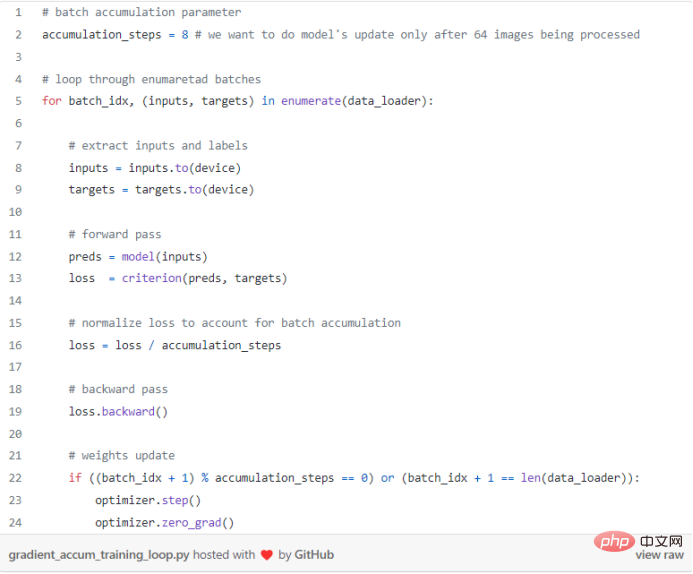
Really beautiful, right? The gradient is calculated when loss.backward() is called and accumulated by PyTorch until it is stopped when optimizer.zero_grad() is called.
Key Point
Some network architectures use dedicated batch operations, such as BatchNorm, when using the same batch size, the results may be slightly different.
Mixed Precision Training
Overview
Mixed precision training refers to converting some or all FP32 parameters into smaller formats such as FP16, TF16 (floating point tensors) or BF16 (floating point bytes) ).
Main advantages
The main advantages of mixed precision training are:
- Reduced memory usage;
- Performance improvements (higher arithmetic intensity or less communication usage);
- #Use dedicated hardware for faster calculations.
Currently I am only interested in the first advantage - reducing memory usage, let's see how to use the PyTorch model to achieve it.
Routine:
# #
As a result, after completing the .half() operation, the model became 2 times smaller. The scaling loss after converting the model to different formats (i.e. BF16, TF16) will be discussed in a subsequent article. Some operations cannot be completed in FP16, such as Softmax. PyTorch can use torch.autocast to handle these special cases.
8-bit optimizer
Increasing model size is an effective way to achieve better performance. However, training large models requires storing the model, gradients, and optimizer state (e.g., Adam's exponential smooth sum and the sum of squares of previous gradients), all of which are stored in a limited amount of available memory.
Downgrade the 32-bit optimizer to the 8-bit optimizer and reduce the range of values from 2³² to only 2⁸=256, which will affect the optimization reserved by the optimizer. The amount of memory makes a huge difference.
The researchers proposed a new 8-bit Adam optimizer. The author of the paper said in the article: "It maintains 32-bit performance to some of the original in memory".
The 8-bit optimizer has three components: (1) block-level quantization, which isolates outliers and distributes errors evenly to every bit; (2) ) Dynamic quantization to quantify small and large values with high accuracy; (3) Stable embedding layer to improve the stability of the word embedding optimization model.
#With these components, optimizations can be performed directly using 8-bit state. Quantize the 8-bit optimizer state to 32 bits, perform the update, and then quantize the state to 8 bits for storage. 8-bit to 32-bit conversion is performed element-wise in registers without the need for slow copies to GPU memory or additional temporary memory to perform quantization and dequantization. For GPUs, this means that the 8-bit optimizer is faster than the regular 32-bit optimizer.
Let’s take a look at the inspiring results after using 8-bit Adam:

As you can see, using quantized Adam saves about 8.5 GB of GPU memory, which looks pretty awesome!
#After understanding its usability, let’s take a look at how to implement it in python.
The Bitsandbytes package provided by Facebook is a lightweight wrapper around CUDA custom functions, encapsulating the 8-bit optimizer and quantization function, using it The use of 8-bit Adam can be realized.
Routine:
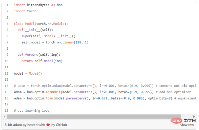
##As mentioned above, the use of the quantization optimizer is very simple and the results are good.
Based on all the above methods, fine-tune GPT-2-XL on the GPU.
Finally, after mastering the above methods, use these methods to solve practical problems and fine-tune the GPT-2-XL model with 1.5 billion parameters. Apparently there's no way to load it onto an NVIDIA GeForce RTX 3060 GPU with 12 GB of RAM. List all methods that can be used:
- Gradient checkpoint;
- Mixed precision training (I set up a trick: use two of the same model Sample. First, load it onto the GPU with .half and name it gpu_model; secondly, on the CPU, name it cpu_model. After evaluating the GPU model, load the gradient of gpu_model into cpu_model and run the optimizer. step(), load the updated parameters into gpu_model);
- Use batch_size=64, minibatch_size=4 gradient accumulation, which needs to be scaled by accumulation_steps Loss;
- 8-bit Adam optimizer.
Use all the above methods and check the code:
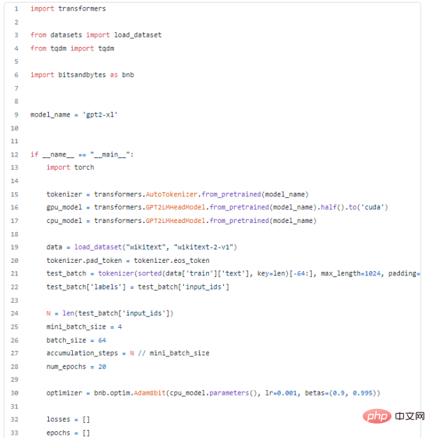
After using all the above methods, I realized the fine-tuning of the 16GB GPT-2-XL model on the GPU, which is amazing!
Conclusion
In this blog, the key concepts of efficient use of memory are given, which is applicable to many A difficult task, as mentioned above. Other concepts will be discussed in subsequent articles. Thank you very much for taking the time to read this article!
The above is the detailed content of How to fine-tune very large models with limited GPU resources. For more information, please follow other related articles on the PHP Chinese website!

Hot AI Tools

Undresser.AI Undress
AI-powered app for creating realistic nude photos

AI Clothes Remover
Online AI tool for removing clothes from photos.

Undress AI Tool
Undress images for free

Clothoff.io
AI clothes remover

AI Hentai Generator
Generate AI Hentai for free.

Hot Article

Hot Tools

Notepad++7.3.1
Easy-to-use and free code editor

SublimeText3 Chinese version
Chinese version, very easy to use

Zend Studio 13.0.1
Powerful PHP integrated development environment

Dreamweaver CS6
Visual web development tools

SublimeText3 Mac version
God-level code editing software (SublimeText3)

Hot Topics
 1385
1385
 52
52
 The world's most powerful open source MoE model is here, with Chinese capabilities comparable to GPT-4, and the price is only nearly one percent of GPT-4-Turbo
May 07, 2024 pm 04:13 PM
Imagine an artificial intelligence model that not only has the ability to surpass traditional computing, but also achieves more efficient performance at a lower cost. This is not science fiction, DeepSeek-V2[1], the world’s most powerful open source MoE model is here. DeepSeek-V2 is a powerful mixture of experts (MoE) language model with the characteristics of economical training and efficient inference. It consists of 236B parameters, 21B of which are used to activate each marker. Compared with DeepSeek67B, DeepSeek-V2 has stronger performance, while saving 42.5% of training costs, reducing KV cache by 93.3%, and increasing the maximum generation throughput to 5.76 times. DeepSeek is a company exploring general artificial intelligence
 Slow Cellular Data Internet Speeds on iPhone: Fixes
May 03, 2024 pm 09:01 PM
Facing lag, slow mobile data connection on iPhone? Typically, the strength of cellular internet on your phone depends on several factors such as region, cellular network type, roaming type, etc. There are some things you can do to get a faster, more reliable cellular Internet connection. Fix 1 – Force Restart iPhone Sometimes, force restarting your device just resets a lot of things, including the cellular connection. Step 1 – Just press the volume up key once and release. Next, press the Volume Down key and release it again. Step 2 – The next part of the process is to hold the button on the right side. Let the iPhone finish restarting. Enable cellular data and check network speed. Check again Fix 2 – Change data mode While 5G offers better network speeds, it works better when the signal is weaker
 Hello, electric Atlas! Boston Dynamics robot comes back to life, 180-degree weird moves scare Musk
Apr 18, 2024 pm 07:58 PM
Boston Dynamics Atlas officially enters the era of electric robots! Yesterday, the hydraulic Atlas just "tearfully" withdrew from the stage of history. Today, Boston Dynamics announced that the electric Atlas is on the job. It seems that in the field of commercial humanoid robots, Boston Dynamics is determined to compete with Tesla. After the new video was released, it had already been viewed by more than one million people in just ten hours. The old people leave and new roles appear. This is a historical necessity. There is no doubt that this year is the explosive year of humanoid robots. Netizens commented: The advancement of robots has made this year's opening ceremony look like a human, and the degree of freedom is far greater than that of humans. But is this really not a horror movie? At the beginning of the video, Atlas is lying calmly on the ground, seemingly on his back. What follows is jaw-dropping
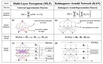 KAN, which replaces MLP, has been extended to convolution by open source projects
Jun 01, 2024 pm 10:03 PM
Earlier this month, researchers from MIT and other institutions proposed a very promising alternative to MLP - KAN. KAN outperforms MLP in terms of accuracy and interpretability. And it can outperform MLP running with a larger number of parameters with a very small number of parameters. For example, the authors stated that they used KAN to reproduce DeepMind's results with a smaller network and a higher degree of automation. Specifically, DeepMind's MLP has about 300,000 parameters, while KAN only has about 200 parameters. KAN has a strong mathematical foundation like MLP. MLP is based on the universal approximation theorem, while KAN is based on the Kolmogorov-Arnold representation theorem. As shown in the figure below, KAN has
 The vitality of super intelligence awakens! But with the arrival of self-updating AI, mothers no longer have to worry about data bottlenecks
Apr 29, 2024 pm 06:55 PM
I cry to death. The world is madly building big models. The data on the Internet is not enough. It is not enough at all. The training model looks like "The Hunger Games", and AI researchers around the world are worrying about how to feed these data voracious eaters. This problem is particularly prominent in multi-modal tasks. At a time when nothing could be done, a start-up team from the Department of Renmin University of China used its own new model to become the first in China to make "model-generated data feed itself" a reality. Moreover, it is a two-pronged approach on the understanding side and the generation side. Both sides can generate high-quality, multi-modal new data and provide data feedback to the model itself. What is a model? Awaker 1.0, a large multi-modal model that just appeared on the Zhongguancun Forum. Who is the team? Sophon engine. Founded by Gao Yizhao, a doctoral student at Renmin University’s Hillhouse School of Artificial Intelligence.
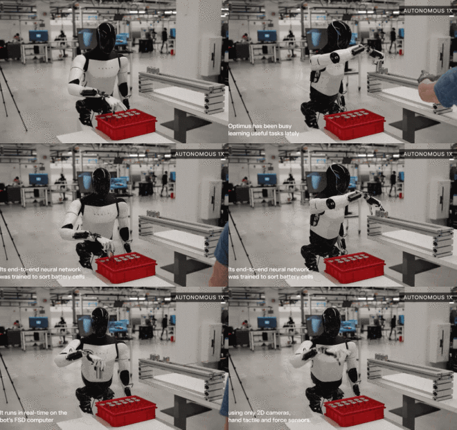 Tesla robots work in factories, Musk: The degree of freedom of hands will reach 22 this year!
May 06, 2024 pm 04:13 PM
The latest video of Tesla's robot Optimus is released, and it can already work in the factory. At normal speed, it sorts batteries (Tesla's 4680 batteries) like this: The official also released what it looks like at 20x speed - on a small "workstation", picking and picking and picking: This time it is released One of the highlights of the video is that Optimus completes this work in the factory, completely autonomously, without human intervention throughout the process. And from the perspective of Optimus, it can also pick up and place the crooked battery, focusing on automatic error correction: Regarding Optimus's hand, NVIDIA scientist Jim Fan gave a high evaluation: Optimus's hand is the world's five-fingered robot. One of the most dexterous. Its hands are not only tactile
 FisheyeDetNet: the first target detection algorithm based on fisheye camera
Apr 26, 2024 am 11:37 AM
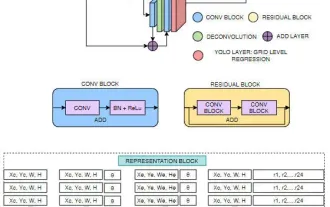
Target detection is a relatively mature problem in autonomous driving systems, among which pedestrian detection is one of the earliest algorithms to be deployed. Very comprehensive research has been carried out in most papers. However, distance perception using fisheye cameras for surround view is relatively less studied. Due to large radial distortion, standard bounding box representation is difficult to implement in fisheye cameras. To alleviate the above description, we explore extended bounding box, ellipse, and general polygon designs into polar/angular representations and define an instance segmentation mIOU metric to analyze these representations. The proposed model fisheyeDetNet with polygonal shape outperforms other models and simultaneously achieves 49.5% mAP on the Valeo fisheye camera dataset for autonomous driving
 The U.S. Air Force showcases its first AI fighter jet with high profile! The minister personally conducted the test drive without interfering during the whole process, and 100,000 lines of code were tested for 21 times.
May 07, 2024 pm 05:00 PM
Recently, the military circle has been overwhelmed by the news: US military fighter jets can now complete fully automatic air combat using AI. Yes, just recently, the US military’s AI fighter jet was made public for the first time and the mystery was unveiled. The full name of this fighter is the Variable Stability Simulator Test Aircraft (VISTA). It was personally flown by the Secretary of the US Air Force to simulate a one-on-one air battle. On May 2, U.S. Air Force Secretary Frank Kendall took off in an X-62AVISTA at Edwards Air Force Base. Note that during the one-hour flight, all flight actions were completed autonomously by AI! Kendall said - "For the past few decades, we have been thinking about the unlimited potential of autonomous air-to-air combat, but it has always seemed out of reach." However now,


