Ten commonly used loss function explanations and Python code implementations

What is the loss function?

The loss function is an algorithm that measures the degree of fit between the model and the data. A loss function is a way of measuring the difference between actual measurements and predicted values. The higher the value of the loss function, the more incorrect the prediction is, and the lower the value of the loss function, the closer the prediction is to the true value. The loss function is calculated for each individual observation (data point). The function that averages the values ​​of all loss functions is called the cost function. A simpler understanding is that the loss function is for a single sample, while the cost function is for all samples.

Loss functions and metrics

Some loss functions can also be used as evaluation metrics. But loss functions and metrics have different purposes. While metrics are used to evaluate the final model and compare the performance of different models, the loss function is used during the model building phase as an optimizer for the model being created. The loss function guides the model on how to minimize the error.

That is to say, the loss function knows how the model is trained, and the measurement index explains the performance of the model.

Why use a loss function?

Since the loss function measures the difference between the predicted value and the actual value, they can be used to guide the improvement of the model when training the model (usually gradient descent method). In the process of building the model, if the weight of the feature changes and gets better or worse predictions, it is necessary to use the loss function to judge whether the weight of the feature in the model needs to be changed, and the direction of change.

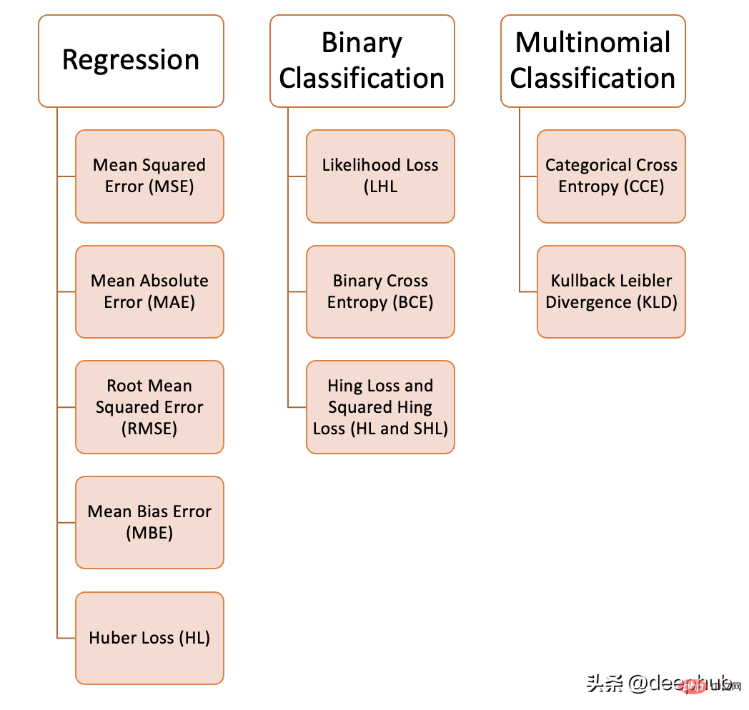
We can use a variety of loss functions in machine learning, depending on the type of problem we are trying to solve, the data quality and distribution, and the algorithm we use. The following figure shows the 10 we have compiled Common loss functions:

Regression problem

1. Mean square error (MSE)

Mean square error refers to all predicted values and the true values, and average them. Often used in regression problems.

def MSE (y, y_predicted):sq_error = (y_predicted - y) ** 2sum_sq_error = np.sum(sq_error)mse = sum_sq_error/y.sizereturn mse

2. Mean absolute error (MAE)

is calculated as the average of the absolute differences between the predicted value and the true value. This is a better measurement than mean squared error when the data has outliers.

def MAE (y, y_predicted):error = y_predicted - yabsolute_error = np.absolute(error)total_absolute_error = np.sum(absolute_error)mae = total_absolute_error/y.sizereturn mae

3. Root mean square error (RMSE)

This loss function is the square root of the mean square error. This is an ideal approach if we don't want to punish larger errors.

def RMSE (y, y_predicted):sq_error = (y_predicted - y) ** 2total_sq_error = np.sum(sq_error)mse = total_sq_error/y.sizermse = math.sqrt(mse)return rmse

4. Mean deviation error (MBE)

is similar to the mean absolute error but does not seek the absolute value. The disadvantage of this loss function is that negative and positive errors can cancel each other out, so it is better to apply it when the researcher knows that the error only goes in one direction.

def MBE (y, y_predicted):error = y_predicted - ytotal_error = np.sum(error)mbe = total_error/y.sizereturn mbe

5. Huber loss

The Huber loss function combines the advantages of mean absolute error (MAE) and mean square error (MSE). This is because Hubber loss is a function with two branches. One branch is applied to MAEs that match expected values, and the other branch is applied to outliers. The general function of Hubber Loss is:

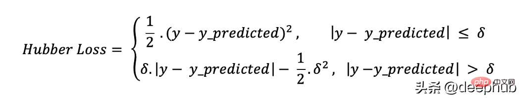
Here

def hubber_loss (y, y_predicted, delta)delta = 1.35 * MAEy_size = y.sizetotal_error = 0for i in range (y_size):erro = np.absolute(y_predicted[i] - y[i])if error < delta:hubber_error = (error * error) / 2else:hubber_error = (delta * error) / (0.5 * (delta * delta))total_error += hubber_errortotal_hubber_error = total_error/y.sizereturn total_hubber_error

Binary classification

6, Maximum likelihood loss (Likelihood Loss/LHL)

This loss function is mainly used for binary classification problems. The probability of each predicted value is multiplied to obtain a loss value, and the associated cost function is the average of all observed values. Let us take the following example of binary classification where the class is [0] or [1]. If the output probability is equal to or greater than 0.5, the predicted class is [1], otherwise it is [0]. An example of the output probability is as follows:

[0.3, 0.7, 0.8, 0.5, 0.6, 0.4]

The corresponding prediction class is:

[0, 1, 1, 1 , 1 , 0]

while the actual class is:

[0 , 1 , 1 , 0 , 1 , 0]

Now the real class and Output the probability to calculate the loss. If the true class is [1], we use the output probability, if the true class is [0], we use the 1-probability:

((1–0.3) 0.7 0.8 (1–0.5) 0.6 (1– 0.4)) / 6 = 0.65

The Python code is as follows:

def LHL (y, y_predicted):likelihood_loss = (y * y_predicted) + ((1-y) * (y_predicted))total_likelihood_loss = np.sum(likelihood_loss)lhl = - total_likelihood_loss / y.sizereturn lhl

7. Binary Cross Entropy (BCE)

This function is a correction of the logarithmic likelihood loss . Stacking sequences of numbers can penalize highly confident but incorrect predictions. The general formula of the binary cross-entropy loss function is:

— (y . log (p) (1 — y) . ​​log (1 — p))

Let’s continue using the above example Values:

Output probability = [0.3, 0.7, 0.8, 0.5, 0.6, 0.4]

Actual class = [0, 1, 1, 0, 1, 0]

— (0 . log (0.3) (1–0) . log (1–0.3)) = 0.155

— (1 . log(0.7) + (1–1) . log (0.3)) = 0.155

— (1 . log(0.8) + (1–1) . log (0.2)) = 0.097

— (0 . log (0.5) + (1–0) . log (1–0.5)) = 0.301

— (1 . log(0.6) + (1–1) . log (0.4)) = 0.222

— (0 . log (0.4) + (1–0) . log (1–0.4)) = 0.222

那么代价函数的结果为：

(0.155 + 0.155 + 0.097 + 0.301 + 0.222 + 0.222) / 6 = 0.192

Python的代码如下：

def BCE (y, y_predicted):ce_loss = y*(np.log(y_predicted))+(1-y)*(np.log(1-y_predicted))total_ce = np.sum(ce_loss)bce = - total_ce/y.sizereturn bce

8、Hinge Loss 和 Squared Hinge Loss (HL and SHL)

Hinge Loss被翻译成铰链损失或者合页损失，这里还是以英文为准。

Hinge Loss主要用于支持向量机模型的评估。错误的预测和不太自信的正确预测都会受到惩罚。 所以一般损失函数是：

l(y) = max (0 , 1 — t . y)

这里的t是真实结果用[1]或[-1]表示。

使用Hinge Loss的类应该是[1]或[-1](不是[0])。为了在Hinge loss函数中不被惩罚，一个观测不仅需要正确分类而且到超平面的距离应该大于margin(一个自信的正确预测)。如果我们想进一步惩罚更高的误差，我们可以用与MSE类似的方法平方Hinge损失,也就是Squared Hinge Loss。

如果你对SVM比较熟悉，应该还记得在SVM中，超平面的边缘（margin）越高，则某一预测就越有信心。如果这块不熟悉，则看看这个可视化的例子:

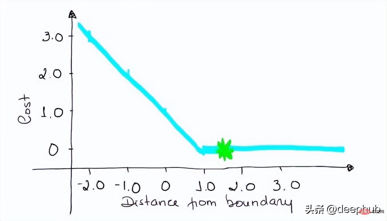
如果一个预测的结果是1.5，并且真正的类是[1]，损失将是0(零)，因为模型是高度自信的。

loss= Max (0,1 - 1* 1.5) = Max (0， -0.5) = 0

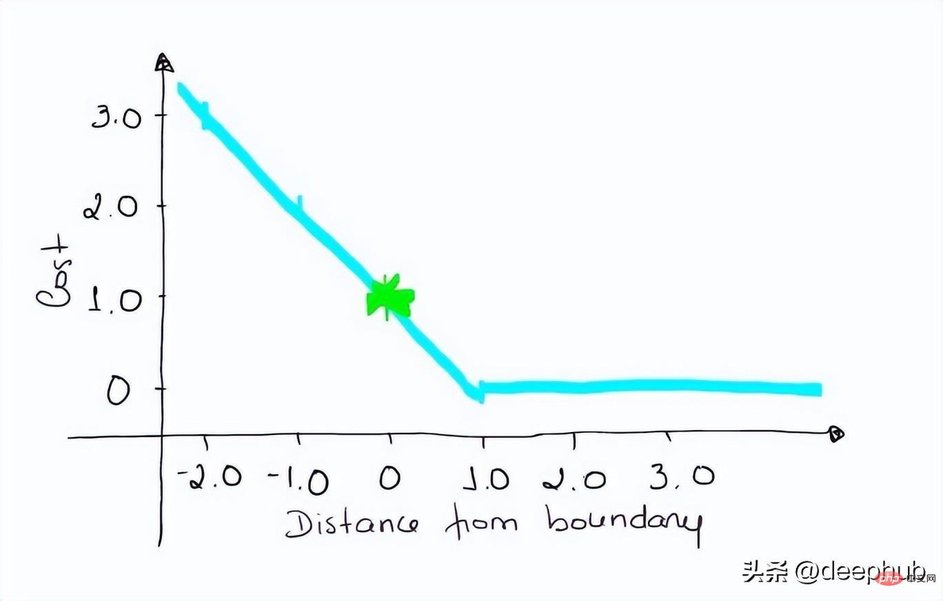
如果一个观测结果为0(0)，则表示该观测处于边界(超平面)，真实的类为[-1]。损失为1，模型既不正确也不错误，可信度很低。

loss = max (0 , 1–(-1) * 0) = max (0 , 1) = 1

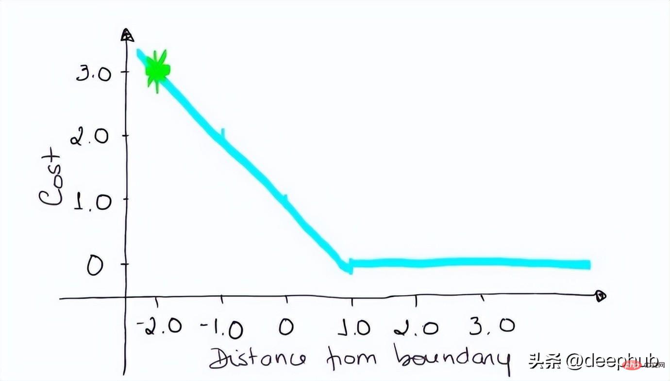
如果一次观测结果为2，但分类错误(乘以[-1])，则距离为-2。损失是3(非常高)，因为我们的模型对错误的决策非常有信心（这个是绝不能容忍的）。

loss = max (0 , 1 — (-1) . 2) = max (0 , 1+2) = max (0 , 3) = 3

python代码如下：

#Hinge Lossdef Hinge (y, y_predicted):hinge_loss = np.sum(max(0 , 1 - (y_predicted * y)))return hinge_loss#Squared Hinge Lossdef SqHinge (y, y_predicted):sq_hinge_loss = max (0 , 1 - (y_predicted * y)) ** 2total_sq_hinge_loss = np.sum(sq_hinge_loss)return total_sq_hinge_loss

多分类

9、交叉熵（CE）

在多分类中，我们使用与二元交叉熵类似的公式，但有一个额外的步骤。首先需要计算每一对[y, y_predicted]的损失，一般公式为：

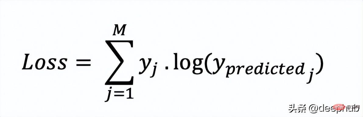
如果我们有三个类，其中单个[y, y_predicted]对的输出是：

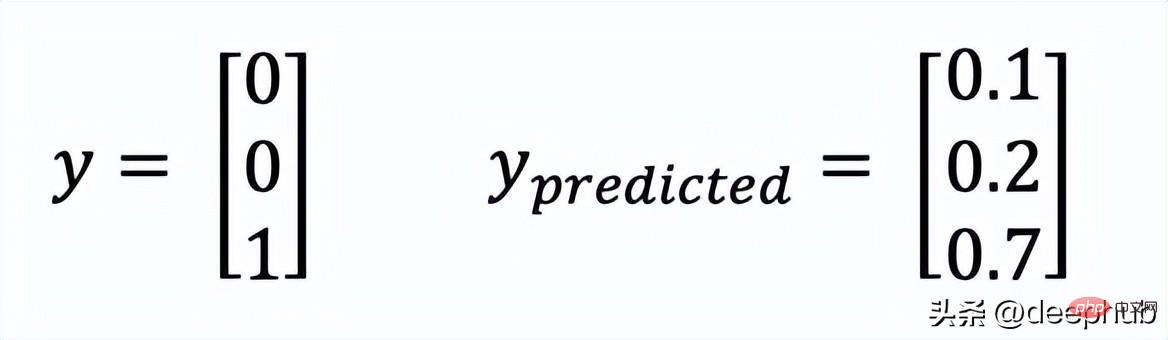
这里实际的类3（也就是值=1的部分），我们的模型对真正的类是3的信任度是0.7。计算这损失如下：

Loss = 0 . log (0.1) + 0 . log (0.2) + 1 . log (0.7) = -0.155

为了得到代价函数的值，我们需要计算所有单个配对的损失，然后将它们相加最后乘以[-1/样本数量]。代价函数由下式给出：

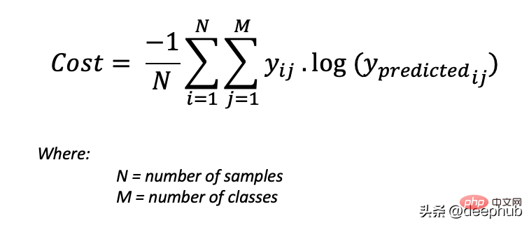
使用上面的例子，如果我们的第二对：

Loss = 0 . log (0.4) + 1. log (0.4) + 0. log (0.2) = -0.40

那么成本函数计算如下：

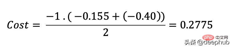
使用Python的代码示例可以更容易理解：

def CCE (y, y_predicted):cce_class = y * (np.log(y_predicted))sum_totalpair_cce = np.sum(cce_class)cce = - sum_totalpair_cce / y.sizereturn cce

10、Kullback-Leibler 散度 (KLD)

又被简化称为KL散度，它类似于分类交叉熵，但考虑了观测值发生的概率。 如果我们的类不平衡，它特别有用。

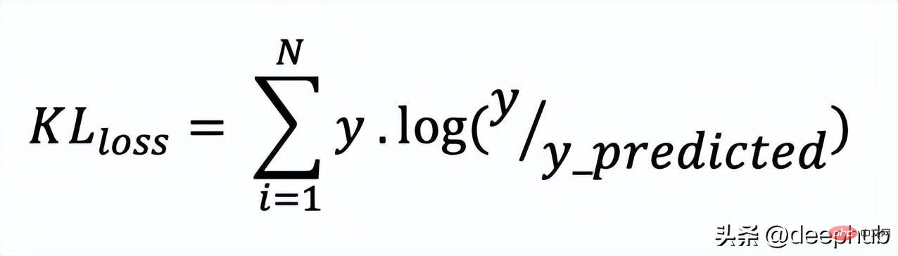
def KL (y, y_predicted):kl = y * (np.log(y / y_predicted))total_kl = np.sum(kl)return total_kl

以上就是常见的10个损失函数，希望对你有所帮助。

The above is the detailed content of Ten commonly used loss function explanations and Python code implementations. For more information, please follow other related articles on the PHP Chinese website!