How to create a drop-down list with symbols in Excel
Creating a drop-down list in an Excel worksheet is easy, as long as it is a regular drop-down menu. But what if you have to make it special by adding a special symbol, or make it even more special by adding some text as well as symbols? Ok, sounds interesting but wondering if this is possible? What's an answer you don't know when Geek Page is here to help?
This article is all about creating dropdown menus with symbols as well as symbols and text. Hope you enjoyed reading this article!
Also read: How to add a drop-down menu in Microsoft Excel
Part 1: Create a drop-down list with only symbols
To create a drop-down menu with symbols, We first need to create a list of sources from which to get the symbols to populate the dropdown menu.
Let's see how to create a symbol source list and how to use this source list to populate a drop-down menu.
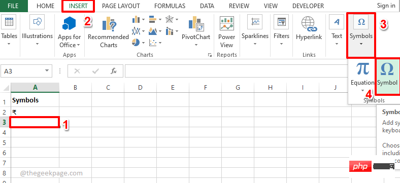
Step 1: First, clickthe cell where you want to insert the first symbol.
With the cell selected, click the INSERT tab at the top and then click the button named Symbols.
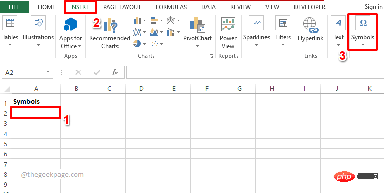
Step 2: Now, from the list of options available under Symbols, click on the Symbol option.
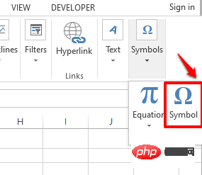
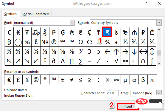
Step 3: You can now see all the special symbols that can be inserted into your Excel worksheet.
Note: You can do some filtering using the Subset drop-down menu in the Sign window.
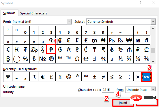
Click on the symbol you want to insert, and then click the "Insert " button.
In the example below, I have chosen to insert a symbol called Indian Rupee Sign.
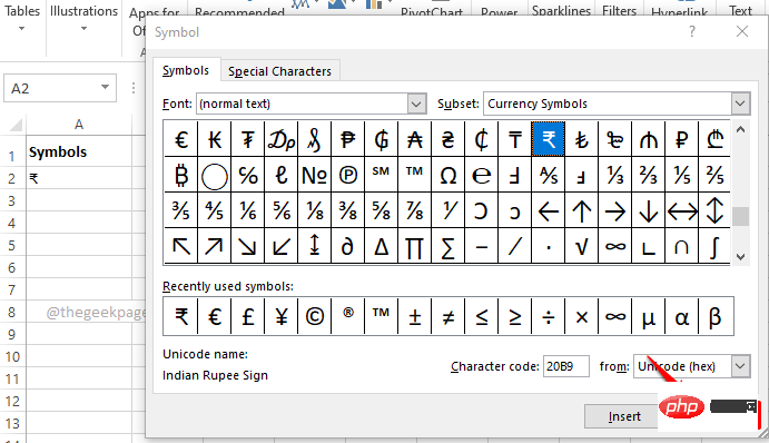
Step 4: You can now see the inserted symbol in the background. Click the Close button to close the symbol window.
Step 5: Now let’s add the second symbol to our source list. To do this, Select the second cell where you want to insert the second symbol, preferably directly below the first symbol.
Now as before, click on the INSERT tab at the top, click on the drop-down menu called Symbols, then click on the Symbol option.
Step 6: You can now select the symbol you want to insert the into. If you want to insert multiple symbols into the same cell, please select the first symbol, click the "Insert" button, select the second symbol, click the "Insert" button again, and so on.
After inserting all the symbols you need, click the Close button.
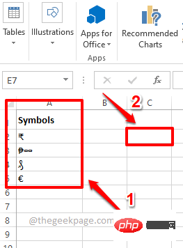
In the example below, I inserted 2 symbols .
Step 7: Again, I added 2 more lines to the source list containing the symbols.
After creating the source list, click the cell where you want to create the drop-down menu.
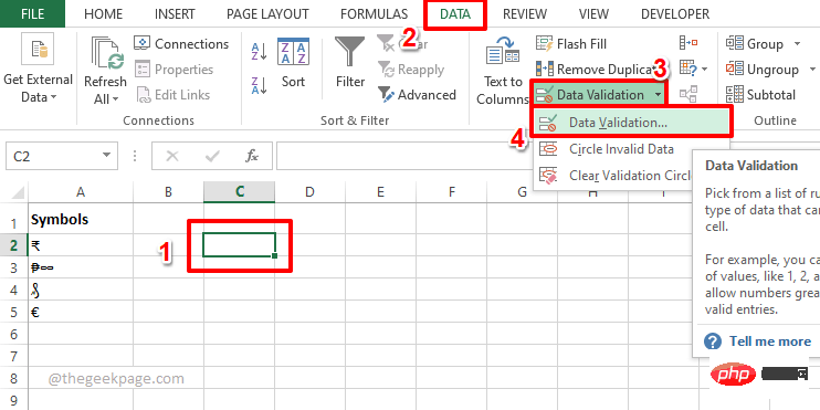
Step 8: Make sure the cell in which you want to create the symbol drop-down menu is selected.
Next, click on the Data tab in the top ribbon. Now click on the Data Validation drop-down menu and click on the Data Validation option.
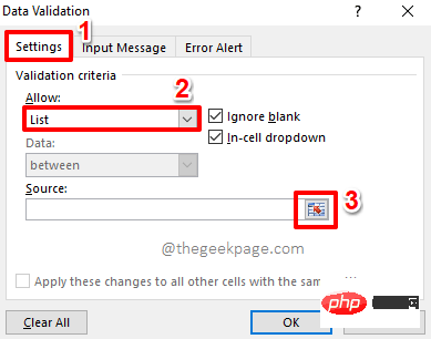
Step 9: In the "Data Verification" window, first click "Settings" Tab.
Now, select List from the list of available options under the Allow drop-down menu.
Next, click the Minimize icon associated with the Source field to select your symbol source list from the Excel table.
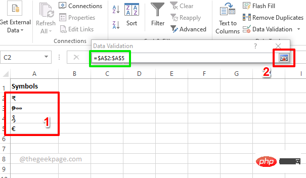
Step 10: Simply click and drag to select the symbol source list you created.
The data validation window will now be automatically populated. Green, marked in the screenshot below.
Click to expand the icon to return to the Data Verification window.
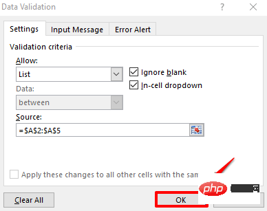
Step 11: Just click the OK button.
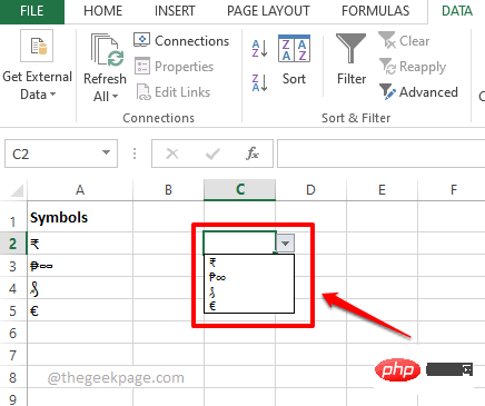
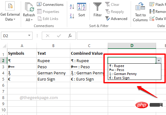
Step 12: Now, if you click on the cell where the drop-down menu is inserted, you can see your own custom symbol drop-down list. enjoy!
Section 2: Creating a Drop-down List Containing Symbols and Text
Now let’s say you want to create a symbol drop-down menu, but you also want to include some text Also associated with your symbol. For this we need to have 2 columns. One for symbols and one for text. We will then merge these 2 columns to make it the source list for a new dropdown containing symbols and text.
First, we need the symbol source list columns that we created in the previous section, and second, we need the text columns that you want to associate with each symbol.
Once you have the two columns ready, follow these steps to connect them perfectly and make a beautiful drop-down menu out of them.
Step 1: Create one more column where your symbols and text will be combined.
Double-click the first cell of the newly created column.
Now, copy and paste the following formula onto it to connect the symbols and text.
=A2 & " : " & B2
Note: A2 is the cell where the first symbol is located, and B2 is the cell where the first text is located. If your value exists in some other cells, replace A2 and B2 with the corresponding cell IDs. Additionally, the : symbols are used as associative operators. You can use any other association, even leave it blank, or skip it entirely.
After writing the formula in one cell, let’s drag the formula down and apply it to all cells below it, in the same column.
Just click the small square in the lower right corner of the cell where the formula is applied and drag it down.
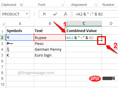
Step 2: Viola, your symbols and text are now merged. Now let's create a dropdown menu using this column.
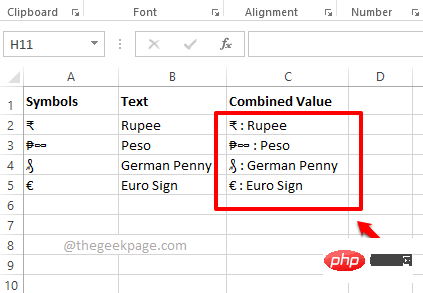
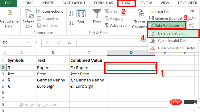
Step 3: First click the cell in which you want to create the drop-down menu.
Click theData tab on the top ribbon, click the Data Validation drop-down menu, then click Data Validation from the available menu options options.
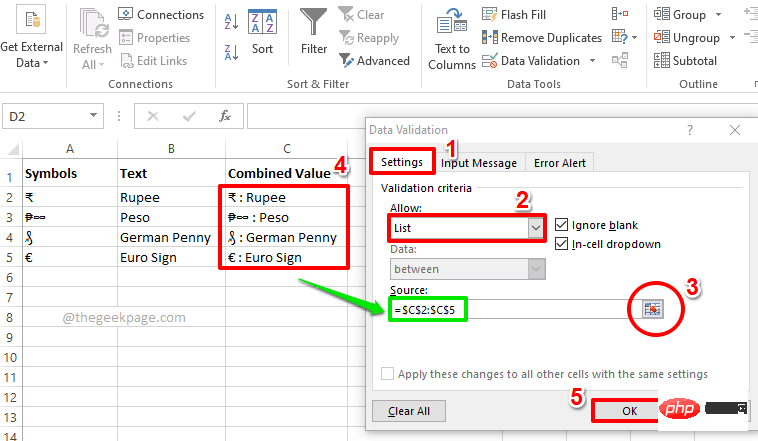
Step 4: In the "Data Verification" window, first click "Settings"Tab. From the Allow drop-down menu, click the List option.
Now, just like in the previous section, use theminimize and expand icons on the source field to select The symbol and text are associated with the list, which is basically the column named combination value in the screenshot below.
Click theOK button after completion.
Step 5: That’s it. You can now show off your new drop-down menu, complete with text and symbols. enjoy!
The above is the detailed content of How to create a drop-down list with symbols in Excel. For more information, please follow other related articles on the PHP Chinese website!

Hot AI Tools

Undresser.AI Undress
AI-powered app for creating realistic nude photos

AI Clothes Remover
Online AI tool for removing clothes from photos.

Undress AI Tool
Undress images for free

Clothoff.io
AI clothes remover

AI Hentai Generator
Generate AI Hentai for free.

Hot Article

Hot Tools

Notepad++7.3.1
Easy-to-use and free code editor

SublimeText3 Chinese version
Chinese version, very easy to use

Zend Studio 13.0.1
Powerful PHP integrated development environment

Dreamweaver CS6
Visual web development tools

SublimeText3 Mac version
God-level code editing software (SublimeText3)

Hot Topics
 1378
1378
 52
52
 How to make drop-down menu in WPS table
Mar 21, 2024 pm 01:31 PM
How to make the WPS table drop-down menu: After selecting the cell where you want to set the drop-down menu, click "Data", "Validity" in sequence, and then make the corresponding settings in the pop-up dialog box to pull down our menu. As a powerful office software, WPS has the ability to edit documents, statistical data tables, etc., which provides a lot of convenience for many people who need to deal with text, data, etc. In order to skillfully use WPS software to provide us with a lot of convenience, we need to be able to master various very basic operations of WPS software. In this article, the editor will share with you how to use WPS software. Perform drop-down menu operations in the WPS table that appears. After opening the WPS form, first select the
 How to prevent Excel from removing leading zeros
Feb 29, 2024 am 10:00 AM
Is it frustrating to automatically remove leading zeros from Excel workbooks? When you enter a number into a cell, Excel often removes the leading zeros in front of the number. By default, it treats cell entries that lack explicit formatting as numeric values. Leading zeros are generally considered irrelevant in number formats and are therefore omitted. Additionally, leading zeros can cause problems in certain numerical operations. Therefore, zeros are automatically removed. This article will teach you how to retain leading zeros in Excel to ensure that the entered numeric data such as account numbers, zip codes, phone numbers, etc. are in the correct format. In Excel, how to allow numbers to have zeros in front of them? You can preserve leading zeros of numbers in an Excel workbook, there are several methods to choose from. You can set the cell by
 VUE3 quick start: using Vue.js instructions to switch tabs
Jun 15, 2023 pm 11:45 PM
This article aims to help beginners quickly get started with Vue.js3 and achieve a simple tab switching effect. Vue.js is a popular JavaScript framework that can be used to build reusable components, easily manage the state of your application, and handle user interface interactions. Vue.js3 is the latest version of the framework. Compared with previous versions, it has undergone major changes, but the basic principles have not changed. In this article, we will use Vue.js instructions to implement the tab switching effect, with the purpose of making readers familiar with Vue.js
 WPS divides one cell into two
Mar 20, 2024 pm 06:00 PM
WPS software is an indispensable helper for text and document processing. In practical applications, it is often necessary to operate in cells to process text and documents. There is a lot of knowledge about cells. Today, let me introduce the specific steps on how to divide a cell into two in WPS. 1. First, we open the WPS table that needs to be edited and select the cell document that needs to be divided into two cells. 2. Click to open "Column" in the data. 3. Then select "Fixed Width" in the pop-up window and click "Next". 4. In the pop-up window, click where you want to separate columns and press Enter to confirm. Draw inferences from one example. If you need to change it to 3, you can also change the number to 3. 5. Then click Finish. 6. There is another way
 How to sum cells in multiple worksheets in Excel
Feb 19, 2024 pm 01:57 PM
This article will demonstrate how to sum cells in multiple worksheets in Excel. Microsoft Excel is a powerful spreadsheet program used for data management. When working with data, you may need to sum across multiple cells. This guide will show you how to achieve this easily. How to sum cells in multiple worksheets in Excel When summing cells in multiple worksheets in Excel, you may encounter the following two situations: Adding a single cell value in a range of cells Adding Values We will cover both methods here. Adding a single cell value across multiple worksheets in Excel We collected a sample number containing the sales of 6 different companies for four consecutive months (from January to April)
 Implement the drop-down menu effect in WeChat applet
Nov 21, 2023 pm 03:03 PM
To implement the drop-down menu effect in WeChat Mini Programs, specific code examples are required. With the popularity of mobile Internet, WeChat Mini Programs have become an important part of Internet development, and more and more people have begun to pay attention to and use WeChat Mini Programs. The development of WeChat mini programs is simpler and faster than traditional APP development, but it also requires mastering certain development skills. In the development of WeChat mini programs, drop-down menus are a common UI component, achieving a better user experience. This article will introduce in detail how to implement the drop-down menu effect in the WeChat applet and provide practical
 Example of new features in PHP8: How to use type declarations and code to strengthen data validation?
Sep 12, 2023 pm 01:21 PM
Example of new features in PHP8: How to use type declarations and code to strengthen data validation? Introduction: With the release of PHP8, developers have welcomed a series of new features and improvements. One of the most exciting is the ability for type declarations and code to enforce data validation. This article will take some practical examples to introduce how to use these new features to strengthen data validation and improve code readability and maintainability. Advantages of type declaration: Before PHP7, the type of variables could be changed at will, which brought great difficulties to data verification.
 Excel keeps changing numbers to latest date; changing dates to random numbers
Feb 27, 2024 pm 02:28 PM
If you encounter the problem of numbers being automatically changed to dates in Excel, or dates turning into random numbers, this article will provide solutions. Some users reported that when they entered numbers, the numbers automatically turned into dates. This problem is usually caused by cell formatting. Excel keeps changing numbers to latest If numbers in Microsoft Excel keep changing to dates, you can fix this problem by formatting the cells as text. Insert an apostrophe before the number. Use Paste Special. 1] Format cells as text To prevent Excel from automatically adjusting number formats, you first need to change the format of the relevant cells to text. Here are the simple steps to do this: First, numerically select all


