Handwriting regression trees from scratch using Python
For the sake of simplicity, recursion will be used to create tree nodes. Although recursion is not a perfect implementation, it is the most intuitive for explaining the principle.
First import the library
import pandas as pd
import numpy as np
import matplotlib.pyplot as plt
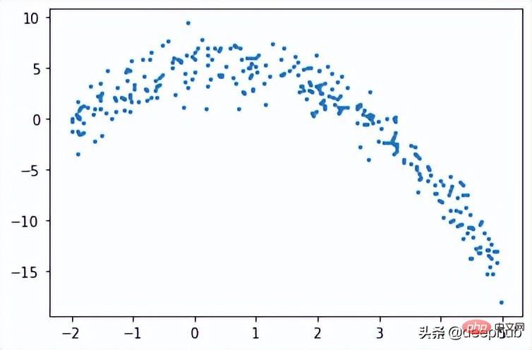
First we need to create the training data, our data will have an independent variable (x) and a dependent variable (y) and use numpy to add Gaussian to the correlated value Noise can be expressed mathematically as

here is noise. The code is shown below.
def f(x):
mu, sigma = 0, 1.5
return -x**2 + x + 5 + np.random.normal(mu, sigma, 1)
num_points = 300
np.random.seed(1)

x = np.random.uniform(-2, 5, num_points)
y = np.array( [f(i) for i in x] )
plt.scatter(x, y, s = 5)
Regression tree
In regression tree, numerical data is predicted by creating a tree of multiple nodes. The figure below shows an example of the tree structure of a regression tree, where each node has its threshold used to divide the data.
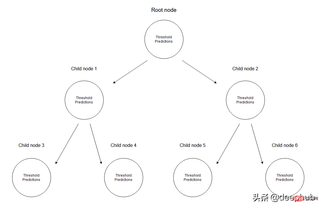
#Given a set of data, the input values will reach the leaf nodes through the corresponding specifications. All input values reaching node M can be represented by subsets of X. Mathematically, let us express this situation in terms of a function that gives 1 if a given input value reaches node M and 0 otherwise.

Find the threshold that splits the data: Iterate over the training data by selecting 2 consecutive points at each step and calculating their average. The calculated mean divides the data into two thresholds.
First let's consider random thresholds to demonstrate any given situation.
threshold = 1.5
low = np.take(y, np.where(x < threshold))
high = np.take(y, np.where(x > threshold))
plt.scatter(x, y, s = 5, label = 'Data')
plt.plot([threshold]*2, [-16, 10], 'b--', label = 'Threshold line')
plt.plot([-2, threshold], [low.mean()]*2, 'r--', label = 'Left child prediction line')
plt.plot([threshold, 5], [high.mean()]*2, 'r--', label = 'Right child prediction line')
plt.plot([-2, 5], [y.mean()]*2, 'g--', label = 'Node prediction line')
plt.legend()

The blue vertical line represents a single threshold, which we assume is the mean of any two points and will be used to divide the data later.
Our first prediction for this problem is the average (green horizontal line) of all training data (y-axis). And the two red lines are the predictions of the child nodes to be created.
It's obvious that none of these averages represent our data well, but their differences are also obvious: the master node prediction (green line) gets the mean of all training data, which we divide into 2 Child nodes, these 2 child nodes have their own predictions (red line). Compared with the green line, these two child nodes better represent their corresponding training data. A regression tree will continuously split the data into 2 parts - creating 2 child nodes from each node until a given stopping value is reached (which is the minimum amount of data a node can have). It stops the tree building process early, which we call a pre-pruned tree.
Why is there an early stopping mechanism? If we were to continue assigning until a node has only one value, this creates an overfitting scenario where each training data can only predict itself.
Description: When the model is complete, it will not use the root node or any intermediate nodes to predict any values; it will use the leaves of the regression tree (which will be the last node of the tree) to make predictions.
To get the threshold that best represents the data for a given threshold, we use the residual sum of squares. It can be mathematically defined as

# Let’s see how this step works.
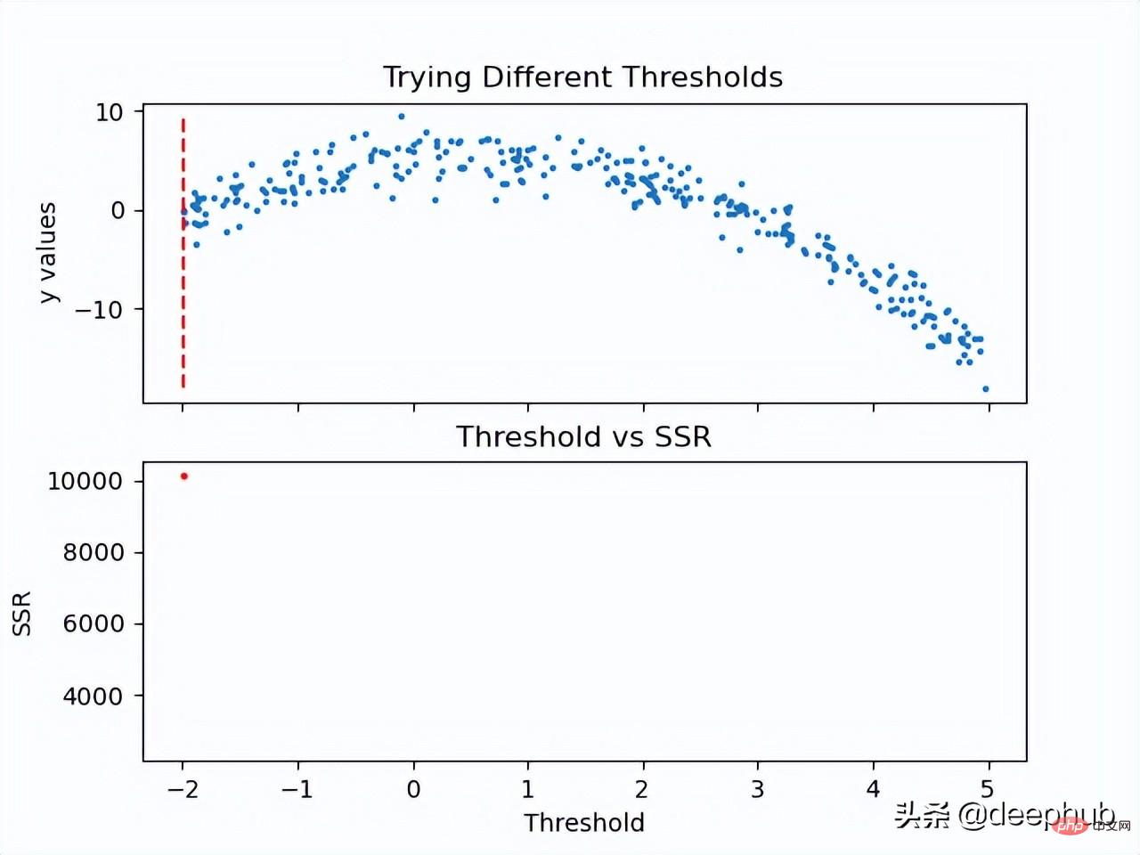
Now that the SSR value of the threshold is calculated, the threshold with the minimum SSR value can be used. Use this threshold to split the training data into two (low and high parts), where the low part will be used to create the left child node and the high part will be used to create the right child node.
def SSR(r, y):
return np.sum( (r - y)**2 )

SSRs, thresholds = [], []
for i in range(len(x) - 1):
threshold = x[i:i+2].mean()

low = np.take(y, np.where(x < threshold))
high = np.take(y, np.where(x > threshold))

guess_low = low.mean()
guess_high = high.mean()

SSRs.append(SSR(low, guess_low) + SSR(high, guess_high))
thresholds.append(threshold)

print('Minimum residual is: {:.2f}'.format(min(SSRs)))
print('Corresponding threshold value is: {:.4f}'.format(thresholds[SSRs.index(min(SSRs))]))
在进入下一步之前,我将使用pandas创建一个df,并创建一个用于寻找最佳阈值的方法。所有这些步骤都可以在没有pandas的情况下完成,这里使用他是因为比较方便。
df = pd.DataFrame(zip(x, y.squeeze()), columns = ['x', 'y'])
def find_threshold(df, plot = False):
SSRs, thresholds = [], []
for i in range(len(df) - 1):
threshold = df.x[i:i+2].mean()
low = df[(df.x <= threshold)]
high = df[(df.x > threshold)]
guess_low = low.y.mean()
guess_high = high.y.mean()
SSRs.append(SSR(low.y.to_numpy(), guess_low) + SSR(high.y.to_numpy(), guess_high))
thresholds.append(threshold)

if plot:
plt.scatter(thresholds, SSRs, s = 3)
plt.show()

return thresholds[SSRs.index(min(SSRs))]
创建子节点
在将数据分成两个部分后就可以为低值和高值找到单独的阈值。需要注意的是这里要增加一个停止条件;因为对于每个节点,属于该节点的数据集中的点会变少,所以我们为每个节点定义了最小数据点数量。如果不这样做,每个节点将只使用一个训练值进行预测,会导致过拟合。
可以递归地创建节点,我们定义了一个名为TreeNode的类,它将存储节点应该存储的每一个值。使用这个类我们首先创建根,同时计算它的阈值和预测值。然后递归地创建它的子节点,其中每个子节点类都存储在父类的left或right属性中。
在下面的create_nodes方法中,首先将给定的df分成两部分。然后检查是否有足够的数据单独创建左右节点。如果(对于其中任何一个)有足够的数据点,我们计算阈值并使用它创建一个子节点,用这个新节点作为树再次调用create_nodes方法。
class TreeNode():
def __init__(self, threshold, pred):
self.threshold = threshold
self.pred = pred
self.left = None
self.right = None
def create_nodes(tree, df, stop):
low = df[df.x <= tree.threshold]
high = df[df.x > tree.threshold]

if len(low) > stop:
threshold = find_threshold(low)
tree.left = TreeNode(threshold, low.y.mean())
create_nodes(tree.left, low, stop)

if len(high) > stop:
threshold = find_threshold(high)
tree.right = TreeNode(threshold, high.y.mean())
create_nodes(tree.right, high, stop)

threshold = find_threshold(df)
tree = TreeNode(threshold, df.y.mean())
create_nodes(tree, df, 5)
这个方法在第一棵树上进行了修改,因为它不需要返回任何东西。虽然递归函数通常不是这样写的(不返回),但因为不需要返回值,所以当没有激活if语句时,不做任何操作。
在完成后可以检查此树结构,查看它是否创建了一些可以拟合数据的节点。 这里将手动选择第一个节点及其对根阈值的预测。
plt.scatter(x, y, s = 0.5, label = 'Data')
plt.plot([tree.threshold]*2, [-16, 10], 'r--',
label = 'Root threshold')
plt.plot([tree.right.threshold]*2, [-16, 10], 'g--',
label = 'Right node threshold')
plt.plot([tree.threshold, tree.right.threshold],
[tree.right.left.pred]*2,
'g', label = 'Right node prediction')
plt.plot([tree.left.threshold]*2, [-16, 10], 'm--',
label = 'Left node threshold')
plt.plot([tree.left.threshold, tree.threshold],
[tree.left.right.pred]*2,
'm', label = 'Left node prediction')
plt.plot([tree.left.left.threshold]*2, [-16, 10], 'k--',
label = 'Second Left node threshold')
plt.legend()
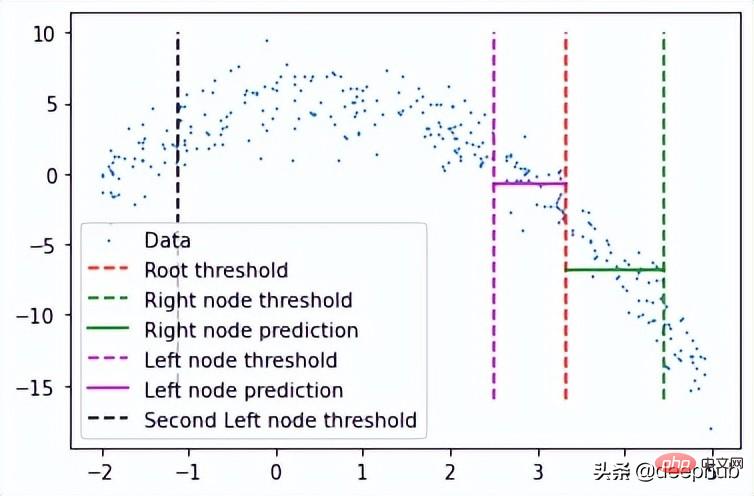
这里看到了两个预测:
- 第一个左节点对高值的预测(高于其阈值)
- 第一个右节点对低值(低于其阈值)的预测
这里我手动剪切了预测线的宽度,因为如果给定的x值达到了这些节点中的任何一个,则将以属于该节点的所有x值的平均值表示,这也意味着没有其他x值参与 在该节点的预测中(希望有意义)。
这种树形结构远不止两个节点那么简单,所以我们可以通过如下调用它的子节点来检查一个特定的叶子节点。
tree.left.right.left.left
这当然意味着这里有一个向下4个子结点长的分支,但它可以在树的另一个分支上深入得多。
预测
我们可以创建一个预测方法来预测任何给定的值。
def predict(x):
curr_node = tree
result = None
while True:
if x <= curr_node.threshold:
if curr_node.left: curr_node = curr_node.left
else:
break
elif x > curr_node.threshold:
if curr_node.right: curr_node = curr_node.right
else:
break

return curr_node.pred
预测方法做的是沿着树向下,通过比较我们的输入和每个叶子的阈值。如果输入值大于阈值,则转到右叶,如果小于阈值,则转到左叶,以此类推,直到到达任何底部叶子节点。然后使用该节点自身的预测值进行预测,并与其阈值进行最后的比较。
使用x = 3进行测试(在创建数据时,可以使用上面所写的函数计算实际值。-3**2+3+5 = -1,这是期望值),我们得到:
predict(3)
# -1.23741
计算误差
这里用相对平方误差验证数据

def RSE(y, g):
return sum(np.square(y - g)) / sum(np.square(y - 1 / len(y)*sum(y)))
x_val = np.random.uniform(-2, 5, 50)
y_val = np.array( [f(i) for i in x_val] ).squeeze()
tr_preds = np.array( [predict(i) for i in df.x] )
val_preds = np.array( [predict(i) for i in x_val] )
print('Training error: {:.4f}'.format(RSE(df.y, tr_preds)))
print('Validation error: {:.4f}'.format(RSE(y_val, val_preds)))可以看到误差并不大,结果如下

概括的步骤

更深入的模型
一个更适合回归树模型的数据:因为我们的数据是多项式生成的数据,所以使用多项式回归模型可以更好地拟合。我们更换一下训练数据,把新函数设为

def f(x):
mu, sigma = 0, 0.5
if x < 3: return 1 + np.random.normal(mu, sigma, 1)
elif x >= 3 and x < 6: return 9 + np.random.normal(mu, sigma, 1)
elif x >= 6: return 5 + np.random.normal(mu, sigma, 1)

np.random.seed(1)

x = np.random.uniform(0, 10, num_points)
y = np.array( [f(i) for i in x] )
plt.scatter(x, y, s = 5)
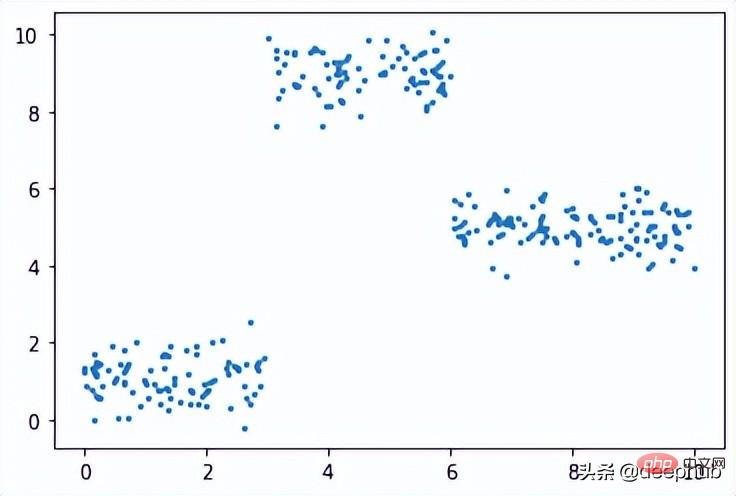
在此数据集上运行了上面的所有相同过程,结果如下

比我们从多项式数据中获得的误差低。
最后共享一下上面动图的代码:
import pandas as pd
import numpy as np
import matplotlib.pyplot as plt
from matplotlib.animation import FuncAnimation
#===================================================Create Data
def f(x):
mu, sigma = 0, 1.5
return -x**2 + x + 5 + np.random.normal(mu, sigma, 1)
np.random.seed(1)

x = np.random.uniform(-2, 5, 300)
y = np.array( [f(i) for i in x] )
p = x.argsort()
x = x[p]
y = y[p]
#===================================================Calculate Thresholds
def SSR(r, y): #send numpy array
return np.sum( (r - y)**2 )
SSRs, thresholds = [], []
for i in range(len(x) - 1):
threshold = x[i:i+2].mean()

low = np.take(y, np.where(x < threshold))
high = np.take(y, np.where(x > threshold))

guess_low = low.mean()
guess_high = high.mean()

SSRs.append(SSR(low, guess_low) + SSR(high, guess_high))
thresholds.append(threshold)
#===================================================Animated Plot
fig, (ax1, ax2) = plt.subplots(2,1, sharex = True)
x_data, y_data = [], []
x_data2, y_data2 = [], []
ln, = ax1.plot([], [], 'r--')
ln2, = ax2.plot(thresholds, SSRs, 'ro', markersize = 2)
line = [ln, ln2]
def init():
ax1.scatter(x, y, s = 3)
ax1.title.set_text('Trying Different Thresholds')
ax2.title.set_text('Threshold vs SSR')
ax1.set_ylabel('y values')
ax2.set_xlabel('Threshold')
ax2.set_ylabel('SSR')
return line
def update(frame):
x_data = [x[frame:frame+2].mean()] * 2
y_data = [min(y), max(y)]
line[0].set_data(x_data, y_data)
x_data2.append(thresholds[frame])
y_data2.append(SSRs[frame])
line[1].set_data(x_data2, y_data2)
return line
ani = FuncAnimation(fig, update, frames = 298,
init_func = init, blit = True)
plt.show()The above is the detailed content of Handwriting regression trees from scratch using Python. For more information, please follow other related articles on the PHP Chinese website!

Hot AI Tools

Undresser.AI Undress
AI-powered app for creating realistic nude photos

AI Clothes Remover
Online AI tool for removing clothes from photos.

Undress AI Tool
Undress images for free

Clothoff.io
AI clothes remover

AI Hentai Generator
Generate AI Hentai for free.

Hot Article

Hot Tools

Notepad++7.3.1
Easy-to-use and free code editor

SublimeText3 Chinese version
Chinese version, very easy to use

Zend Studio 13.0.1
Powerful PHP integrated development environment

Dreamweaver CS6
Visual web development tools

SublimeText3 Mac version
God-level code editing software (SublimeText3)

Hot Topics
 1381
1381
 52
52
 PHP and Python: Code Examples and Comparison
Apr 15, 2025 am 12:07 AM
PHP and Python have their own advantages and disadvantages, and the choice depends on project needs and personal preferences. 1.PHP is suitable for rapid development and maintenance of large-scale web applications. 2. Python dominates the field of data science and machine learning.
 How to train PyTorch model on CentOS
Apr 14, 2025 pm 03:03 PM
Efficient training of PyTorch models on CentOS systems requires steps, and this article will provide detailed guides. 1. Environment preparation: Python and dependency installation: CentOS system usually preinstalls Python, but the version may be older. It is recommended to use yum or dnf to install Python 3 and upgrade pip: sudoyumupdatepython3 (or sudodnfupdatepython3), pip3install--upgradepip. CUDA and cuDNN (GPU acceleration): If you use NVIDIAGPU, you need to install CUDATool
 How is the GPU support for PyTorch on CentOS
Apr 14, 2025 pm 06:48 PM
Enable PyTorch GPU acceleration on CentOS system requires the installation of CUDA, cuDNN and GPU versions of PyTorch. The following steps will guide you through the process: CUDA and cuDNN installation determine CUDA version compatibility: Use the nvidia-smi command to view the CUDA version supported by your NVIDIA graphics card. For example, your MX450 graphics card may support CUDA11.1 or higher. Download and install CUDAToolkit: Visit the official website of NVIDIACUDAToolkit and download and install the corresponding version according to the highest CUDA version supported by your graphics card. Install cuDNN library:
 Detailed explanation of docker principle
Apr 14, 2025 pm 11:57 PM
Docker uses Linux kernel features to provide an efficient and isolated application running environment. Its working principle is as follows: 1. The mirror is used as a read-only template, which contains everything you need to run the application; 2. The Union File System (UnionFS) stacks multiple file systems, only storing the differences, saving space and speeding up; 3. The daemon manages the mirrors and containers, and the client uses them for interaction; 4. Namespaces and cgroups implement container isolation and resource limitations; 5. Multiple network modes support container interconnection. Only by understanding these core concepts can you better utilize Docker.
 Python vs. JavaScript: Community, Libraries, and Resources
Apr 15, 2025 am 12:16 AM
Python and JavaScript have their own advantages and disadvantages in terms of community, libraries and resources. 1) The Python community is friendly and suitable for beginners, but the front-end development resources are not as rich as JavaScript. 2) Python is powerful in data science and machine learning libraries, while JavaScript is better in front-end development libraries and frameworks. 3) Both have rich learning resources, but Python is suitable for starting with official documents, while JavaScript is better with MDNWebDocs. The choice should be based on project needs and personal interests.
 How to choose the PyTorch version under CentOS
Apr 14, 2025 pm 02:51 PM
When selecting a PyTorch version under CentOS, the following key factors need to be considered: 1. CUDA version compatibility GPU support: If you have NVIDIA GPU and want to utilize GPU acceleration, you need to choose PyTorch that supports the corresponding CUDA version. You can view the CUDA version supported by running the nvidia-smi command. CPU version: If you don't have a GPU or don't want to use a GPU, you can choose a CPU version of PyTorch. 2. Python version PyTorch
 MiniOpen Centos compatibility
Apr 14, 2025 pm 05:45 PM
MinIO Object Storage: High-performance deployment under CentOS system MinIO is a high-performance, distributed object storage system developed based on the Go language, compatible with AmazonS3. It supports a variety of client languages, including Java, Python, JavaScript, and Go. This article will briefly introduce the installation and compatibility of MinIO on CentOS systems. CentOS version compatibility MinIO has been verified on multiple CentOS versions, including but not limited to: CentOS7.9: Provides a complete installation guide covering cluster configuration, environment preparation, configuration file settings, disk partitioning, and MinI
 How to operate distributed training of PyTorch on CentOS
Apr 14, 2025 pm 06:36 PM
PyTorch distributed training on CentOS system requires the following steps: PyTorch installation: The premise is that Python and pip are installed in CentOS system. Depending on your CUDA version, get the appropriate installation command from the PyTorch official website. For CPU-only training, you can use the following command: pipinstalltorchtorchvisiontorchaudio If you need GPU support, make sure that the corresponding version of CUDA and cuDNN are installed and use the corresponding PyTorch version for installation. Distributed environment configuration: Distributed training usually requires multiple machines or single-machine multiple GPUs. Place


