

How to apply superscript and subscript formatting options in Microsoft Excel

A superscript is a character or characters, either letters or numbers, that you need to set slightly higher than a normal line of text. For example, if you need to write 1st, the letters st need to be slightly higher than the characters 1. Likewise, a subscript is a group of characters or a single character and needs to be set slightly lower than normal text level. For example, when you write a chemical formula, you need to place the numbers below the normal line of characters. The following screenshots show some examples of superscript and subscript formatting.

Although it may seem like a daunting task, applying superscript and subscript formatting to your text is actually quite simple. In this article, we will explain in some simple steps how to easily format text using superscript or subscript. Hope you enjoyed reading this article.
How to apply superscript formatting in Excel
Step 1:Double-click the cell containing the text to which you want to apply superscript formatting. Once in edit mode, click and selectthe text you want to set as superscript.

Step 2: With the text selected, right-click on it and select "Format Cells " option.

Step 3: In the Format Cells window, under the Effects section, select the The option Superscript corresponds to the checkbox. Click the OK button when finished.

Step 4: If you look at the formatted text now, you can see that the superscript formatting has been successfully applied.

Step 5: There is no shortcut to batch format superscript text. You need to apply superscript formatting one by one. Below is a screenshot of the entire column with superscript formatting.

How to apply subscript formatting in Excel
Step 1: Just like in superscript formatting, firstDouble-click the cell and select the text to which you want to apply the subscript format .

Step 2: Now right click on the selected text and click Click the "Cell Format" option.

Step 3: Next, select the checkbox corresponding to the Subscript option andClick the OK button.

Step 4: If you look at the Excel worksheet now, you can see that the subscript formatting has been successfully applied.

Step 5: Again, we don’t have the option to batch apply subscript formatting. So, you have to do it manually one by one as shown in the screenshot below.

The above is the detailed content of How to apply superscript and subscript formatting options in Microsoft Excel. For more information, please follow other related articles on the PHP Chinese website!

Hot AI Tools

Undresser.AI Undress
AI-powered app for creating realistic nude photos

AI Clothes Remover
Online AI tool for removing clothes from photos.

Undress AI Tool
Undress images for free

Clothoff.io
AI clothes remover

AI Hentai Generator
Generate AI Hentai for free.

Hot Article
Hot Tools

Notepad++7.3.1
Easy-to-use and free code editor

SublimeText3 Chinese version
Chinese version, very easy to use

Zend Studio 13.0.1
Powerful PHP integrated development environment

Dreamweaver CS6
Visual web development tools

SublimeText3 Mac version
God-level code editing software (SublimeText3)
Hot Topics
 1377
1377
 52
52

 How to set the print area in Google Sheets?
May 08, 2023 pm 01:28 PM
How to set the print area in Google Sheets?
May 08, 2023 pm 01:28 PM
How to Set GoogleSheets Print Area in Print Preview Google Sheets allows you to print spreadsheets with three different print areas. You can choose to print the entire spreadsheet, including each individual worksheet you create. Alternatively, you can choose to print a single worksheet. Finally, you can only print a portion of the cells you select. This is the smallest print area you can create since you could theoretically select individual cells for printing. The easiest way to set it up is to use the built-in Google Sheets print preview menu. You can view this content using Google Sheets in a web browser on your PC, Mac, or Chromebook. To set up Google
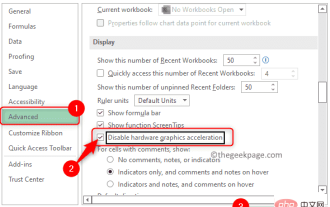 How to solve out of memory problem in Microsoft Excel?
Apr 22, 2023 am 10:04 AM
How to solve out of memory problem in Microsoft Excel?
Apr 22, 2023 am 10:04 AM
Microsoft Excel is a popular program used for creating worksheets, data entry operations, creating graphs and charts, etc. It helps users organize their data and perform analysis on this data. As can be seen, all versions of the Excel application have memory issues. Many users have reported seeing the error message "Insufficient memory to run Microsoft Excel. Please close other applications and try again." when trying to open Excel on their Windows PC. Once this error is displayed, users will not be able to use MSExcel as the spreadsheet will not open. Some users reported problems opening Excel downloaded from any email client
 5 Tips to Fix Stdole32.tlb Excel Error in Windows 11
May 09, 2023 pm 01:37 PM
5 Tips to Fix Stdole32.tlb Excel Error in Windows 11
May 09, 2023 pm 01:37 PM
When you start Microsoft Word or Microsoft Excel, Windows very tediously tries to set up Office 365. At the end of the process, you may receive a Stdole32.tlbExcel error. Since there are many bugs in the Microsoft Office suite, launching any of its products can sometimes be a nightmare. Microsoft Office is a software that is used regularly. Microsoft Office has been available to consumers since 1990. Starting from Office 1.0 version and developing to Office 365, this
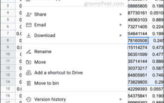
 How to embed a PDF document in an Excel worksheet
May 28, 2023 am 09:17 AM
How to embed a PDF document in an Excel worksheet
May 28, 2023 am 09:17 AM
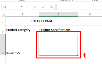
It is usually necessary to insert PDF documents into Excel worksheets. Just like a company's project list, we can instantly append text and character data to Excel cells. But what if you want to attach the solution design for a specific project to its corresponding data row? Well, people often stop and think. Sometimes thinking doesn't work either because the solution isn't simple. Dig deeper into this article to learn how to easily insert multiple PDF documents into an Excel worksheet, along with very specific rows of data. Example Scenario In the example shown in this article, we have a column called ProductCategory that lists a project name in each cell. Another column ProductSpeci
 How to find and delete merged cells in Excel
Apr 20, 2023 pm 11:52 PM
How to find and delete merged cells in Excel
Apr 20, 2023 pm 11:52 PM
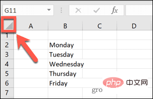
How to Find Merged Cells in Excel on Windows Before you can delete merged cells from your data, you need to find them all. It's easy to do this using Excel's Find and Replace tool. Find merged cells in Excel: Highlight the cells where you want to find merged cells. To select all cells, click in an empty space in the upper left corner of the spreadsheet or press Ctrl+A. Click the Home tab. Click the Find and Select icon. Select Find. Click the Options button. At the end of the FindWhat settings, click Format. Under the Alignment tab, click Merge Cells. It should contain a check mark rather than a line. Click OK to confirm the format
 How to prevent Excel from removing leading zeros
Feb 29, 2024 am 10:00 AM
How to prevent Excel from removing leading zeros
Feb 29, 2024 am 10:00 AM
Is it frustrating to automatically remove leading zeros from Excel workbooks? When you enter a number into a cell, Excel often removes the leading zeros in front of the number. By default, it treats cell entries that lack explicit formatting as numeric values. Leading zeros are generally considered irrelevant in number formats and are therefore omitted. Additionally, leading zeros can cause problems in certain numerical operations. Therefore, zeros are automatically removed. This article will teach you how to retain leading zeros in Excel to ensure that the entered numeric data such as account numbers, zip codes, phone numbers, etc. are in the correct format. In Excel, how to allow numbers to have zeros in front of them? You can preserve leading zeros of numbers in an Excel workbook, there are several methods to choose from. You can set the cell by
 How to reduce Excel file size?
Apr 21, 2023 pm 03:01 PM
How to reduce Excel file size?
Apr 21, 2023 pm 03:01 PM
How to Reduce File Size in Excel by Deleting Worksheets Using multiple worksheets in Excel makes it easier to build a spreadsheet, but the more worksheets you use, the larger the file size. Deleting unnecessary worksheets can help reduce file size. Deleting a worksheet in Excel: Make sure the worksheet you want to delete does not contain any data that is needed or referenced by other worksheets. Right-click on the worksheet tab at the bottom of the screen. Select Delete. The sheet will be deleted - repeat these steps for any other sheets you want to delete. Clear PivotTable Cache PivotTables in Excel are a great way to analyze your data, but they can have a significant impact on the size of your Excel file. This is because, by default
 How to calculate the difference between dates on Google Sheets
Apr 19, 2023 pm 08:07 PM
How to calculate the difference between dates on Google Sheets
Apr 19, 2023 pm 08:07 PM
If you are tasked with working with a spreadsheet containing a large number of dates, calculating the difference between multiple dates can be very frustrating. While the easiest option is to rely on an online date calculator, it may not be the most convenient as you may have to enter the dates one by one into the online tool and then manually copy the results into a spreadsheet. For large numbers of dates, you need a tool that gets the job done more conveniently. Fortunately, Google Sheets allows users to locally calculate the difference between two dates in a spreadsheet. In this post, we will help you calculate the number of days between two dates on Google Sheets using some built-in functions. How to calculate the difference between dates on Google Sheets if you want Google