How to sum values in a column in Microsoft Word
How to find the sum of all values in a column? You might not even say wait until you tell me how you do it. But wait, did I tell you it's not Excel, it's Word? In Excel, everyone knows how to apply a formula function and find the sum of all values in a column. But with Microsoft Word, people often rely on a calculator to find the sum of values, or they import data from Word into Excel, do the calculations, and then put it back into Word. Well, neither solution is ideal for obvious reasons. Wondering what else to do? Would you believe me if I told you that finding the sum of values is easier in Word than in Excel? You have to do it because this is reality!
In this article, we will tell you how to quickly find the sum of all values in a column in Microsoft Word with the help of some built-in features and 2 different solutions. Hope you like it!
Solution 1: Via Layout Tab Data Formulas
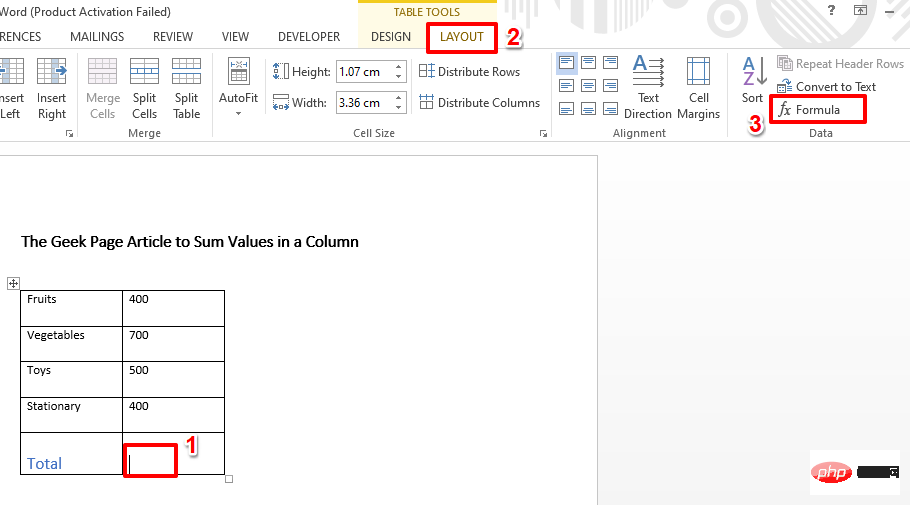
Step 1: Assume you have the following table. We need to find the sum of the values in the second column.
To do this, Click on the cell whose sum value you want to calculate.
Now you will be able to see 2 contextual tabs namely Design and Layout. Click the Layout tab. Next, under the Data section of the LAYOUT tab, click the button named Formula.
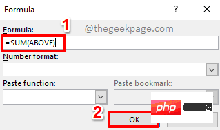
Step 2: Under the "Formula" field in the "Formula" window, has been filled with = SUM(ABOVE) function. If not, just copy and paste it.
After completion, click the OK button.
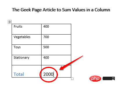
Step 3: That’s it. If you look at the Excel worksheet now, you can see that the sum of the values is calculated and displayed on the cell you selected.
Extra Cookie Section
By default, the sum function will automatically fill in as =SUM(ABOVE). This means, add all the values above the selected cell. You can customize it and set it to =SUM(BELOW) and it will sum up all the values under the selected cell. Likewise, if you use the function =SUM(LEFT), it will sum all values to the left of the selected cell, just like how =SUM(RIGHT) All values on the right side of the cell sum to the same value.
Solution 2: Customize the Quick Access Toolbar
If you often need to find the sum of values in Microsoft Word, then you can add the Sum function to your Quick Access Toolbar. In this case, every time you need to find the sum, you can just click this button on the Quick Access Toolbar. Let's see how to do this.
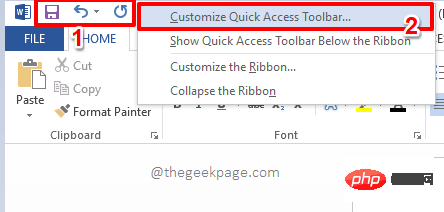
Step 1: Right-click anywhere on the Quick Access Toolbar. From the right-click context menu options, click the Customize Quick Access Toolbar option.
Step 2: In the Word Options window, the left pane will automatically Select Quick Access Toolbar.
In the center pane of the window, click the drop-down arrow icon associated with the option Select a command from .
From the list of available options in the drop-down list, click the option that says All Commands.
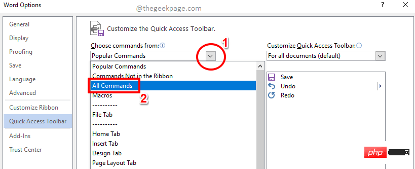
Step 3: Now, Scroll through the list of available options and click on the one that says Sum options. Next click the Add>> button.
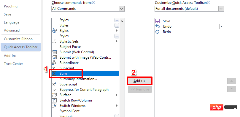
Step 4: Now, the Sum functionality will be added to the right pane of the window. Click the OK button to continue.
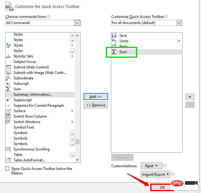
Step 5: The Sum function is now successfully added to the Quick Access Toolbar.
You now simply click the cell where you want to display the sum value and then click on the Quick Access Toolbar The sum button can be used to calculate the sum.
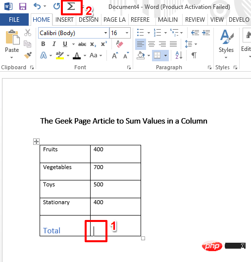
Step 6: Viola! Now you can generate sums with just one click.

The above is the detailed content of How to sum values in a column in Microsoft Word. For more information, please follow other related articles on the PHP Chinese website!

Hot AI Tools

Undresser.AI Undress
AI-powered app for creating realistic nude photos

AI Clothes Remover
Online AI tool for removing clothes from photos.

Undress AI Tool
Undress images for free

Clothoff.io
AI clothes remover

AI Hentai Generator
Generate AI Hentai for free.

Hot Article

Hot Tools

Notepad++7.3.1
Easy-to-use and free code editor

SublimeText3 Chinese version
Chinese version, very easy to use

Zend Studio 13.0.1
Powerful PHP integrated development environment

Dreamweaver CS6
Visual web development tools

SublimeText3 Mac version
God-level code editing software (SublimeText3)

Hot Topics
 Excel found a problem with one or more formula references: How to fix it
Apr 17, 2023 pm 06:58 PM
Use an Error Checking Tool One of the quickest ways to find errors with your Excel spreadsheet is to use an error checking tool. If the tool finds any errors, you can correct them and try saving the file again. However, the tool may not find all types of errors. If the error checking tool doesn't find any errors or fixing them doesn't solve the problem, then you need to try one of the other fixes below. To use the error checking tool in Excel: select the Formulas tab. Click the Error Checking tool. When an error is found, information about the cause of the error will appear in the tool. If it's not needed, fix the error or delete the formula causing the problem. In the Error Checking Tool, click Next to view the next error and repeat the process. When not
 How to add the Quick Launch Toolbar to the taskbar in Windows 11
Apr 14, 2023 pm 02:31 PM
In Windows 10 and Windows 11, the Quick Launch Toolbar is located on the taskbar (before the system tray) and helps users open or launch frequently accessed files, folders, applications, etc. This is a native feature of Windows 10 that allows users to create custom toolbars to access files, folders, and applications. However, in Windows 11, users cannot use this feature. However, it is possible to create and add a Quick Launch Toolbar to access files, folders, and applications that are regularly accessed from the system tray of your Windows 11 PC. Are you looking to use Quick Launch Toolbar on your Windows 11 system then continue reading this article
 How to set the print area in Google Sheets?
May 08, 2023 pm 01:28 PM
How to Set GoogleSheets Print Area in Print Preview Google Sheets allows you to print spreadsheets with three different print areas. You can choose to print the entire spreadsheet, including each individual worksheet you create. Alternatively, you can choose to print a single worksheet. Finally, you can only print a portion of the cells you select. This is the smallest print area you can create since you could theoretically select individual cells for printing. The easiest way to set it up is to use the built-in Google Sheets print preview menu. You can view this content using Google Sheets in a web browser on your PC, Mac, or Chromebook. To set up Google
 How to embed a PDF document in an Excel worksheet
May 28, 2023 am 09:17 AM
It is usually necessary to insert PDF documents into Excel worksheets. Just like a company's project list, we can instantly append text and character data to Excel cells. But what if you want to attach the solution design for a specific project to its corresponding data row? Well, people often stop and think. Sometimes thinking doesn't work either because the solution isn't simple. Dig deeper into this article to learn how to easily insert multiple PDF documents into an Excel worksheet, along with very specific rows of data. Example Scenario In the example shown in this article, we have a column called ProductCategory that lists a project name in each cell. Another column ProductSpeci
 What should I do if there are too many different cell formats that cannot be copied?
Mar 02, 2023 pm 02:46 PM
Solution to the problem that there are too many different cell formats that cannot be copied: 1. Open the EXCEL document, and then enter the content of different formats in several cells; 2. Find the "Format Painter" button in the upper left corner of the Excel page, and then click " "Format Painter" option; 3. Click the left mouse button to set the format to be consistent.
 How to deal with the problem that the toolbar cannot be seen in WPS2019
Mar 27, 2024 pm 02:20 PM
1. As shown in the picture below, after we open a WPS text software, we cannot see the required toolbar or ribbon. This is because we have hidden it. 2. Solution 1: We first click the Show/Hide Ribbon button in the upper right corner of the menu bar to hide or show the ribbon. 3. Click this button to display the ribbon. 4. Method 2: When the ribbon is hidden, we can place the mouse on the name of the ribbon, such as Start and Insert, to display the hidden ribbon. 5. But if we move the mouse to the editing area and do not move the mouse for a long time, as shown in the figure below, the ribbon will automatically hide again. This is because we have turned on the automatic hiding/showing function. 6. At this point we need to click the interface settings button in the upper right corner first. 7. Then click the drop-down menu
 How to remove commas from numeric and text values in Excel
Apr 17, 2023 pm 09:01 PM
On numeric values, on text strings, using commas in the wrong places can really get annoying, even for the biggest Excel geeks. You may even know how to get rid of commas, but the method you know may be time-consuming for you. Well, no matter what your problem is, if it is related to a comma in the wrong place in your Excel worksheet, we can tell you one thing, all your problems will be solved today, right here! Dig deeper into this article to learn how to easily remove commas from numbers and text values in the simplest steps possible. Hope you enjoy reading. Oh, and don’t forget to tell us which method catches your eye the most! Section 1: How to Remove Commas from Numerical Values When a numerical value contains a comma, there are two possible situations:
 How to find and delete merged cells in Excel
Apr 20, 2023 pm 11:52 PM
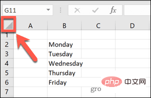
How to Find Merged Cells in Excel on Windows Before you can delete merged cells from your data, you need to find them all. It's easy to do this using Excel's Find and Replace tool. Find merged cells in Excel: Highlight the cells where you want to find merged cells. To select all cells, click in an empty space in the upper left corner of the spreadsheet or press Ctrl+A. Click the Home tab. Click the Find and Select icon. Select Find. Click the Options button. At the end of the FindWhat settings, click Format. Under the Alignment tab, click Merge Cells. It should contain a check mark rather than a line. Click OK to confirm the format


