Ten alternative data processing techniques for Pandas

The techniques compiled in this article are different from the common techniques compiled in 10 Pandas before. You may not use it often, but sometimes when you encounter some very difficult problems, these techniques can help you quickly Solve some uncommon problems.

1. Categorical type

By default, columns with a limited number of options will be assigned the object type. But it's not an efficient choice in terms of memory. We can index these columns and use only references to the objects and not the actual values. Pandas provides a Dtype called Categorical to solve this problem.

For example, it consists of a large data set with image paths. Each row has three columns: anchor, positive, and negative.

If you use Categorical for categorical columns, you can significantly reduce memory usage.

# raw data
 +----------+------------------------+
 |class |filename|
 +----------+------------------------+
 | Bathroom | Bathroombath_1.jpg|
 | Bathroom | Bathroombath_100.jpg|
 | Bathroom | Bathroombath_1003.jpg |
 | Bathroom | Bathroombath_1004.jpg |
 | Bathroom | Bathroombath_1005.jpg |
 +----------+------------------------+

 # target
 +------------------------+------------------------+----------------------------+
 | anchor |positive|negative|
 +------------------------+------------------------+----------------------------+
 | Bathroombath_1.jpg| Bathroombath_100.jpg| Dinningdin_540.jpg|
 | Bathroombath_100.jpg| Bathroombath_1003.jpg | Dinningdin_1593.jpg |
 | Bathroombath_1003.jpg | Bathroombath_1004.jpg | Bedroombed_329.jpg|
 | Bathroombath_1004.jpg | Bathroombath_1005.jpg | Livingroomliving_1030.jpg |
 | Bathroombath_1005.jpg | Bathroombath_1007.jpg | Bedroombed_1240.jpg |
 +------------------------+------------------------+----------------------------+

The value of the filename column will be copied frequently. Therefore, memory usage can be greatly reduced by using Categorical.

Let's read the target data set and see the difference in memory:

triplets.info(memory_usage="deep")

 # Column Non-Null Count Dtype
 # --- ------ -------------- -----
 # 0 anchor 525000 non-null category
 # 1 positive 525000 non-null category
 # 2 negative 525000 non-null category
 # dtypes: category(3)
 # memory usage: 4.6 MB

 # without categories
 triplets_raw.info(memory_usage="deep")

 # Column Non-Null Count Dtype
 # --- ------ -------------- -----
 # 0 anchor 525000 non-null object
 # 1 positive 525000 non-null object
 # 2 negative 525000 non-null object
 # dtypes: object(3)
 # memory usage: 118.1 MB

The difference is very large, and the difference grows non-linearly as the number of repetitions increases.

2. Row-column conversion

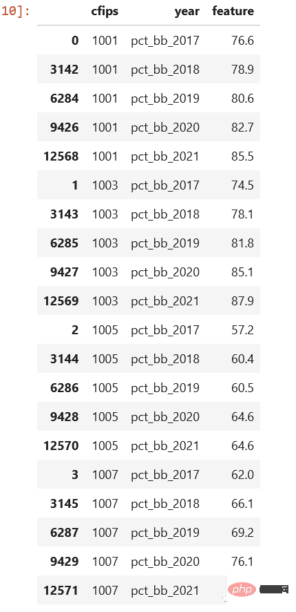
The problem of row-column conversion is often encountered in sql. Pandas sometimes also needs it. Let's take a look at the data set from the Kaggle competition. census_start .csv file:

As you can see, these are saved by year. If there is a column year and pct_bb, and each row has a corresponding value, it will be better A lot, right.

cols = sorted([col for col in original_df.columns
 if col.startswith("pct_bb")])
 df = original_df[(["cfips"] + cols)]
 df = df.melt(id_vars="cfips",
value_vars=cols,
var_name="year",
value_name="feature").sort_values(by=["cfips", "year"])

Look at the result, is this much better:

##3. apply() is very slow

As we introduced last time, it is best not to use this method because it iterates through each row and calls the specified method. But if we have no other choice, is there any way to increase the speed?

You can use packages such as swifter or pandarallew to parallelize the process.

Swifter

import pandas as pd
 import swifter

 def target_function(row):
 return row * 10

 def traditional_way(data):
 data['out'] = data['in'].apply(target_function)

 def swifter_way(data):
 data['out'] = data['in'].swifter.apply(target_function)

Pandaralllel

import pandas as pd
 from pandarallel import pandarallel

 def target_function(row):
 return row * 10

 def traditional_way(data):
 data['out'] = data['in'].apply(target_function)

 def pandarallel_way(data):
 pandarallel.initialize()
 data['out'] = data['in'].parallel_apply(target_function)

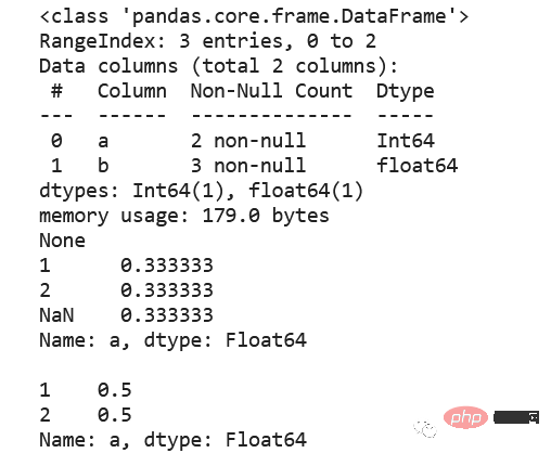
Through multi-threading, the speed of calculation can be improved. Of course, if there is a cluster, it is best to use dask or pyspark

4. Null value, int, Int64

The standard integer data type does not support null value, so it will be automatically converted to a floating point number. So if your data requires null values ​​in integer fields, consider using the Int64 data type as it will use pandas.NA to represent null values.

5. Csv, compression or parquet?

Choose parquet as much as possible. Parquet will retain the data type, so there is no need to specify dtypes when reading data. Parquet files are compressed using snappy by default, so they take up little disk space. Below you can see a few comparisons

|file|size |
 +------------------------+---------+
 | triplets_525k.csv| 38.4 MB |
 | triplets_525k.csv.gzip |4.3 MB |
 | triplets_525k.csv.zip|4.5 MB |
 | triplets_525k.parquet|1.9 MB |
 +------------------------+---------+

Reading parquet requires additional packages, such as pyarrow or fastparquet. chatgpt said that pyarrow is faster than fastparquet, but when I tested on a small data set, fastparquet was faster than pyarrow, but it is recommended to use pyarrow here, because pandas 2.0 also uses this by default.

6, value_counts ()

Calculating relative frequencies, including getting the absolute value, counting, and dividing by the total is complex, but using value_counts, this task can be accomplished more easily, and This method provides the option to include or exclude null values.

df = pd.DataFrame({"a": [1, 2, None], "b": [4., 5.1, 14.02]})
 df["a"] = df["a"].astype("Int64")
 print(df.info())
 print(df["a"].value_counts(normalize=True, dropna=False),
df["a"].value_counts(normalize=True, dropna=True), sep="nn")

Isn’t this much simpler?

7. Modin

Note: Modin is still here testing phase.

Pandas is single-threaded, but Modin can speed up the workflow by scaling pandas. It works particularly well on larger data sets, where pandas can become very slow or Excessive memory usage leads to OOM.

!pip install modin[all]

 import modin.pandas as pd
 df = pd.read_csv("my_dataset.csv")

The following is the architecture diagram of modin’s official website. If you are interested in studying it:

8, extract()

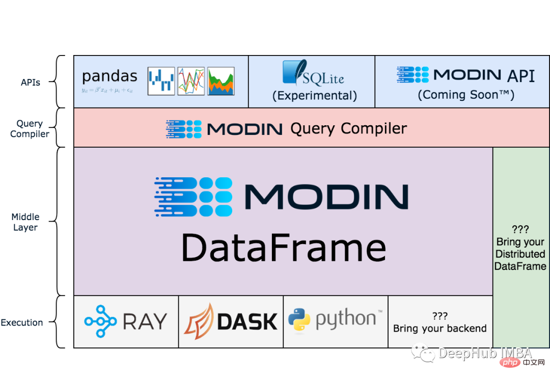
If you often encounter complex semi-structured data and need to separate individual columns from it, you can use this method:

import pandas as pd

 regex = (r'(?P<title>[A-Za-z's]+),'
r'(?P<author>[A-Za-zs']+),'
r'(?P<isbn>[d-]+),'
r'(?P<year>d{4}),'
r'(?P<publisher>.+)')
 addr = pd.Series([
 "The Lost City of Amara,Olivia Garcia,978-1-234567-89-0,2023,HarperCollins",
 "The Alchemist's Daughter,Maxwell Greene,978-0-987654-32-1,2022,Penguin Random House",
 "The Last Voyage of the HMS Endeavour,Jessica Kim,978-5-432109-87-6,2021,Simon & Schuster",
 "The Ghosts of Summer House,Isabella Lee,978-3-456789-12-3,2000,Macmillan Publishers",
 "The Secret of the Blackthorn Manor,Emma Chen,978-9-876543-21-0,2023,Random House Children's Books"
])
 addr.str.extract(regex)

9、读写剪贴板

这个技巧有人一次也用不到，但是有人可能就是需要，比如：在分析中包含PDF文件中的表格时。通常的方法是复制数据，粘贴到Excel中，导出到csv文件中，然后导入Pandas。但是，这里有一个更简单的解决方案:pd.read_clipboard()。我们所需要做的就是复制所需的数据并执行一个方法。

有读就可以写，所以还可以使用to_clipboard()方法导出到剪贴板。

但是要记住，这里的剪贴板是你运行python/jupyter主机的剪切板，并不可能跨主机粘贴，一定不要搞混了。

10、数组列分成多列

假设我们有这样一个数据集，这是一个相当典型的情况:

import pandas as pd
 df = pd.DataFrame({"a": [1, 2, 3],
"b": [4, 5, 6],
"category": [["foo", "bar"], ["foo"], ["qux"]]})

 # let's increase the number of rows in a dataframe
 df = pd.concat([df]*10000, ignore_index=True)

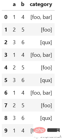
我们想将category分成多列显示，例如下面的

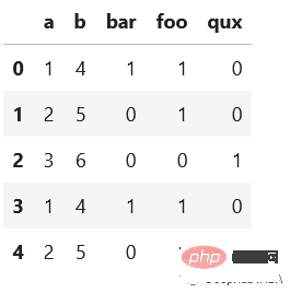
先看看最慢的apply：

def dummies_series_apply(df):
return df.join(df['category'].apply(pd.Series)
.stack()
.str.get_dummies()
.groupby(level=0)
.sum())
.drop("category", axis=1)
 %timeit dummies_series_apply(df.copy())
 #5.96 s ± 66.6 ms per loop (mean ± std. dev. of 7 runs, 1 loop each)

sklearn的MultiLabelBinarizer

from sklearn.preprocessing import MultiLabelBinarizer
 def sklearn_mlb(df):
mlb = MultiLabelBinarizer()
return df.join(pd.DataFrame(mlb.fit_transform(df['category']), columns=mlb.classes_))
.drop("category", axis=1)
 %timeit sklearn_mlb(df.copy())
 #35.1 ms ± 1.31 ms per loop (mean ± std. dev. of 7 runs, 10 loops each)

是不是快了很多，我们还可以使用一般的向量化操作对其求和：

def dummies_vectorized(df):
return pd.get_dummies(df.explode("category"), prefix="cat")
.groupby(["a", "b"])
.sum()
.reset_index()
 %timeit dummies_vectorized(df.copy())
 #29.3 ms ± 1.22 ms per loop (mean ± std. dev. of 7 runs, 10 loops each)

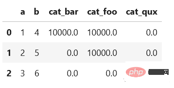
使用第一个方法(在StackOverflow上的回答中非常常见)会给出一个非常慢的结果。而其他两个优化的方法的时间是非常快速的。

总结

我希望每个人都能从这些技巧中学到一些新的东西。重要的是要记住尽可能使用向量化操作而不是apply()。此外，除了csv之外，还有其他有趣的存储数据集的方法。不要忘记使用分类数据类型，它可以节省大量内存。感谢阅读!

The above is the detailed content of Ten alternative data processing techniques for Pandas. For more information, please follow other related articles on the PHP Chinese website!