
 Backend Development
Python Tutorial
Thirty Python functions solve 99% of data processing tasks!
Backend Development
Python Tutorial
Thirty Python functions solve 99% of data processing tasks!
Thirty Python functions solve 99% of data processing tasks!


We know that Pandas is the most widely used data analysis and manipulation library in Python. It provides many functions and methods to quickly solve data processing problems in data analysis.
In order to better master the use of Python functions, I took the customer churn data set as an example to share the 30 most commonly used functions and methods in the data analysis process. The data can be downloaded at the end of the article.
The data is as follows:
import numpy as np
import pandas as pd
df = pd.read_csv("Churn_Modelling.csv")
print(df.shape)
df.columns
Result output
(10000, 14)
Index(['RowNumber', 'CustomerId', 'Surname', 'CreditScore', 'Geography','Gender', 'Age', 'Tenure', 'Balance', 'NumOfProducts', 'HasCrCard','IsActiveMember', 'EstimatedSalary', 'Exited'],dtype='object')
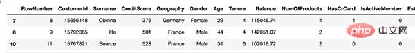
1. Delete column
df.drop(['RowNumber', 'CustomerId', 'Surname', 'CreditScore'], axis=1, inplace=True)
print(df[:2])
print(df.shape)
Result output
Description: "axis ” parameter is set to 1 for columns and 0 for rows. Set the "inplace=True" parameter to True to save changes. We subtracted 4 columns, so the number of columns was reduced from 14 to 10.
GeographyGenderAgeTenureBalanceNumOfProductsHasCrCard
0FranceFemale 42 20.011
 IsActiveMemberEstimatedSalaryExited
0 1101348.88 1
(10000, 10)
2. Select specific columns
We read partial column data from the csv file. The usecols parameter can be used.
df_spec = pd.read_csv("Churn_Modelling.csv", usecols=['Gender', 'Age', 'Tenure', 'Balance'])
df_spec.head()
3.nrows
You can use the nrows parameter to create a data frame containing the first 5000 rows of the csv file. You can also use the skiprows parameter to select lines from the end of the file. Skiprows=5000 means we will skip the first 5000 rows when reading the csv file.
df_partial = pd.read_csv("Churn_Modelling.csv", nrows=5000)
print(df_partial.shape)
4. Sample
After creating the data frame, we may need a small sample to test the data. We can use the n or frac parameter to determine the sample size.
df= pd.read_csv("Churn_Modelling.csv", usecols=['Gender', 'Age', 'Tenure', 'Balance'])
df_sample = df.sample(n=1000)
df_sample2 = df.sample(frac=0.1)
5. Check for missing values
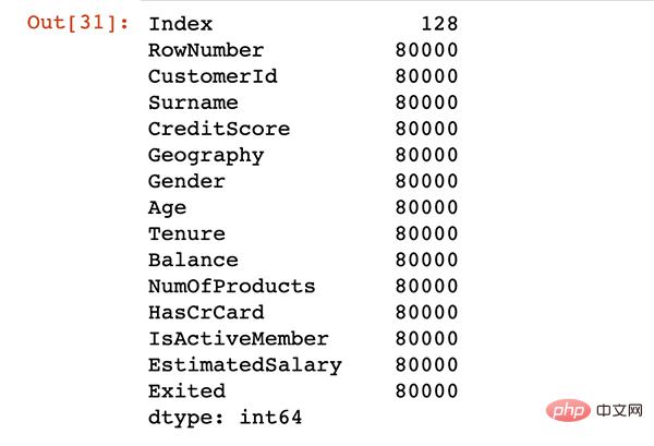
The isna function determines missing values in a data frame. By using isna with the sum function we can see the number of missing values in each column.
df.isna().sum()
6. Use loc and iloc to add missing values
Use loc and iloc to add missing values. The difference between the two is as follows:
- loc: Select with label
- iloc: select index
We first create 20 random indexes for selection.
missing_index = np.random.randint(10000, size=20)
We will use loc to change some values to np.nan (missing values).
df.loc[missing_index, ['Balance','Geography']] = np.nan
20 values are missing in the "Balance" and "Geography" columns. Let's do another example using iloc.
df.iloc[missing_index, -1] = np.nan
7. Fill in missing values
The fillna function is used to fill in missing values. It provides many options. We can use a specific value, an aggregate function such as mean, or the previous or next value.
avg = df['Balance'].mean()
df['Balance'].fillna(value=avg, inplace=True)
fillna The method parameter of the function can be used to fill missing values based on the previous or next value in the column (for example, method="ffill"). It can be very useful for sequential data such as time series.
8. Delete missing values
Another way to deal with missing values is to delete them. The following code will delete rows with any missing values.
df.dropna(axis=0, how='any', inplace=True)
9. Select rows based on conditions
In some cases, we need observations (i.e. rows) that fit certain conditions
france_churn = df[(df.Geography == 'France') & (df.Exited == 1)]
france_churn.Geography.value_counts()
10. Use queries to describe conditions
Query functions provide a more flexible way to pass conditions. We can describe them using strings.
df2 = df.query('80000 < Balance < 100000')
df2 = df.query('80000 < Balance < 100000'
df2 = df.query('80000 < Balance < 100000')
11. Use isin to describe conditions
Conditions may have multiple values. In this case, it's better to use the isin method instead of writing the values individually.
df[df['Tenure'].isin([4,6,9,10])][:3]
12.Groupby Function
Pandas Groupby function is a versatile and easy-to-use function that helps in getting an overview of your data. It makes it easier to explore data sets and reveal underlying relationships between variables.
We will do several examples of group ratio functions. Let's start simple. The following code will group rows based on the combination of Geography and Gender, and then give the average flow of each group
df[['Geography','Gender','Exited']].groupby(['Geography','Gender']).mean()
13.Groupby combined with aggregate functions
agg function allows multiple applications to be applied to the group an aggregate function, with a list of functions passed as arguments.
df[['Geography','Gender','Exited']].groupby(['Geography','Gender']).agg(['mean','count'])
14. Apply different aggregation functions to different groups
df_summary = df[['Geography','Exited','Balance']].groupby('Geography').agg({'Exited':'sum', 'Balance':'mean'})
df_summary.rename(columns={'Exited':'# of churned customers', 'Balance':'Average Balance of Customers'},inplace=True)
In addition, the "NamedAgg function" allows renaming the columns in the aggregation
import pandas as pd
df_summary = df[['Geography','Exited','Balance']].groupby('Geography').agg(Number_of_churned_customers = pd.NamedAgg('Exited', 'sum'),Average_balance_of_customers = pd.NamedAgg('Balance', 'mean'))
print(df_summary)

15.Reset index
Have you noticed the data format in the above picture? We can change this by resetting the index.
print(df_summary.reset_index())

16. Reset and delete the original index
In some cases, we need to reset the index and delete the original index at the same time.
df[['Geography','Exited','Balance']].sample(n=6).reset_index(drop=True)
17. Set specific column as index
We can set any column in the data frame as index.
df_new.set_index('Geography')
18.Insert new column
group = np.random.randint(10, size=6)
df_new['Group'] = group
19.where function
It is used to replace values in rows or columns based on conditions. The default replacement value is NaN, but we can also specify a replacement value.
df_new['Balance'] = df_new['Balance'].where(df_new['Group'] >= 6, 0)
20. Rank Function
The rank function assigns a ranking to a value. Let's create a column that ranks customers based on their balance.
df_new['rank'] = df_new['Balance'].rank(method='first', ascending=False).astype('int')
21. Number of unique values in a column
It comes in handy when working with categorical variables. We may need to check the number of unique categories. We can check the size of the sequence returned by the value count function or use the nunique function.
df.Geography.nunique
22. Memory usage
Using the function memory_usage, these values show the memory in bytes.
df.memory_usage()
23.数据类型转换
默认情况下,分类数据与对象数据类型一起存储。但是,它可能会导致不必要的内存使用,尤其是当分类变量具有较低的基数。
低基数意味着列与行数相比几乎没有唯一值。例如,地理列具有 3 个唯一值和 10000 行。
我们可以通过将其数据类型更改为"类别"来节省内存。
df['Geography'] = df['Geography'].astype('category')
24.替换值
替换函数可用于替换数据帧中的值。
df['Geography'].replace({0:'B1',1:'B2'})
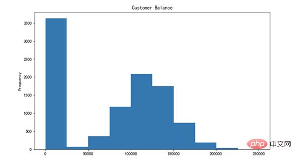
25.绘制直方图
pandas 不是一个数据可视化库,但它使得创建基本绘图变得非常简单。
我发现使用 Pandas 创建基本绘图更容易,而不是使用其他数据可视化库。
让我们创建平衡列的直方图。
26.减少浮点数小数点
pandas 可能会为浮点数显示过多的小数点。我们可以轻松地调整它。
df['Balance'].plot(kind='hist', figsize=(10,6),
title='Customer Balance')
27.更改显示选项
我们可以更改各种参数的默认显示选项,而不是每次手动调整显示选项。
- get_option:返回当前选项
- set_option:更改选项 让我们将小数点的显示选项更改为 2。
pd.set_option("display.precision", 2)
可能要更改的一些其他选项包括:
- max_colwidth:列中显示的最大字符数
- max_columns:要显示的最大列数
- max_rows:要显示的最大行数
28.通过列计算百分比变化
pct_change用于计算序列中值的变化百分比。在计算时间序列或元素顺序数组中更改的百分比时,它很有用。
ser= pd.Series([2,4,5,6,72,4,6,72])
ser.pct_change()
29.基于字符串的筛选
我们可能需要根据文本数据(如客户名称)筛选观测值(行)。我已经在数据帧中添加了df_new名称。

df_new[df_new.Names.str.startswith('Mi')]
我们可能需要根据文本数据(如客户名称)筛选观测值(行)。我已经在数据帧中添加了df_new名称。

30.设置数据样式
我们可以通过使用返回 Style 对象的 Style 属性来实现此目的,它提供了许多用于格式化和显示数据框的选项。例如,我们可以突出显示最小值或最大值。
它还允许应用自定义样式函数。
df_new.style.highlight_max(axis=0, color='darkgreen')

The above is the detailed content of Thirty Python functions solve 99% of data processing tasks!. For more information, please follow other related articles on the PHP Chinese website!

Hot AI Tools

Undresser.AI Undress
AI-powered app for creating realistic nude photos

AI Clothes Remover
Online AI tool for removing clothes from photos.

Undress AI Tool
Undress images for free

Clothoff.io
AI clothes remover

AI Hentai Generator
Generate AI Hentai for free.

Hot Article
Hot Tools

Notepad++7.3.1
Easy-to-use and free code editor

SublimeText3 Chinese version
Chinese version, very easy to use

Zend Studio 13.0.1
Powerful PHP integrated development environment

Dreamweaver CS6
Visual web development tools

SublimeText3 Mac version
God-level code editing software (SublimeText3)
Hot Topics
 1377
1377
 52
52

 Do mysql need to pay
Apr 08, 2025 pm 05:36 PM
Do mysql need to pay
Apr 08, 2025 pm 05:36 PM
MySQL has a free community version and a paid enterprise version. The community version can be used and modified for free, but the support is limited and is suitable for applications with low stability requirements and strong technical capabilities. The Enterprise Edition provides comprehensive commercial support for applications that require a stable, reliable, high-performance database and willing to pay for support. Factors considered when choosing a version include application criticality, budgeting, and technical skills. There is no perfect option, only the most suitable option, and you need to choose carefully according to the specific situation.
 HadiDB: A lightweight, horizontally scalable database in Python
Apr 08, 2025 pm 06:12 PM
HadiDB: A lightweight, horizontally scalable database in Python
Apr 08, 2025 pm 06:12 PM
HadiDB: A lightweight, high-level scalable Python database HadiDB (hadidb) is a lightweight database written in Python, with a high level of scalability. Install HadiDB using pip installation: pipinstallhadidb User Management Create user: createuser() method to create a new user. The authentication() method authenticates the user's identity. fromhadidb.operationimportuseruser_obj=user("admin","admin")user_obj.
 Navicat's method to view MongoDB database password
Apr 08, 2025 pm 09:39 PM
Navicat's method to view MongoDB database password
Apr 08, 2025 pm 09:39 PM
It is impossible to view MongoDB password directly through Navicat because it is stored as hash values. How to retrieve lost passwords: 1. Reset passwords; 2. Check configuration files (may contain hash values); 3. Check codes (may hardcode passwords).
 Does mysql need the internet
Apr 08, 2025 pm 02:18 PM
Does mysql need the internet
Apr 08, 2025 pm 02:18 PM
MySQL can run without network connections for basic data storage and management. However, network connection is required for interaction with other systems, remote access, or using advanced features such as replication and clustering. Additionally, security measures (such as firewalls), performance optimization (choose the right network connection), and data backup are critical to connecting to the Internet.
 Can mysql workbench connect to mariadb
Apr 08, 2025 pm 02:33 PM
Can mysql workbench connect to mariadb
Apr 08, 2025 pm 02:33 PM
MySQL Workbench can connect to MariaDB, provided that the configuration is correct. First select "MariaDB" as the connector type. In the connection configuration, set HOST, PORT, USER, PASSWORD, and DATABASE correctly. When testing the connection, check that the MariaDB service is started, whether the username and password are correct, whether the port number is correct, whether the firewall allows connections, and whether the database exists. In advanced usage, use connection pooling technology to optimize performance. Common errors include insufficient permissions, network connection problems, etc. When debugging errors, carefully analyze error information and use debugging tools. Optimizing network configuration can improve performance
 How to optimize MySQL performance for high-load applications?
Apr 08, 2025 pm 06:03 PM
How to optimize MySQL performance for high-load applications?
Apr 08, 2025 pm 06:03 PM
MySQL database performance optimization guide In resource-intensive applications, MySQL database plays a crucial role and is responsible for managing massive transactions. However, as the scale of application expands, database performance bottlenecks often become a constraint. This article will explore a series of effective MySQL performance optimization strategies to ensure that your application remains efficient and responsive under high loads. We will combine actual cases to explain in-depth key technologies such as indexing, query optimization, database design and caching. 1. Database architecture design and optimized database architecture is the cornerstone of MySQL performance optimization. Here are some core principles: Selecting the right data type and selecting the smallest data type that meets the needs can not only save storage space, but also improve data processing speed.
 How to solve mysql cannot connect to local host
Apr 08, 2025 pm 02:24 PM
How to solve mysql cannot connect to local host
Apr 08, 2025 pm 02:24 PM
The MySQL connection may be due to the following reasons: MySQL service is not started, the firewall intercepts the connection, the port number is incorrect, the user name or password is incorrect, the listening address in my.cnf is improperly configured, etc. The troubleshooting steps include: 1. Check whether the MySQL service is running; 2. Adjust the firewall settings to allow MySQL to listen to port 3306; 3. Confirm that the port number is consistent with the actual port number; 4. Check whether the user name and password are correct; 5. Make sure the bind-address settings in my.cnf are correct.
 How to use AWS Glue crawler with Amazon Athena
Apr 09, 2025 pm 03:09 PM
How to use AWS Glue crawler with Amazon Athena
Apr 09, 2025 pm 03:09 PM
As a data professional, you need to process large amounts of data from various sources. This can pose challenges to data management and analysis. Fortunately, two AWS services can help: AWS Glue and Amazon Athena.
