 Backend Development
 Python Tutorial
 Use Python to implement the top ten classic sorting algorithms
Use Python to implement the top ten classic sorting algorithms

10 classic sorting algorithms include bubble sort, selection sort, quick sort, merge sort, heap sort, insertion sort, Hill sort, counting sort, bucket sort, radix sort, etc. .
Of course, there are some other sorting algorithms, and you can continue to study them.
01Bubble Sort
Bubble Sort is a relatively simple sorting algorithm. It repeatedly visits the elements to be sorted and compares two adjacent elements in turn. If they are in the wrong order, swap them around until no more elements need to be swapped and the sorting is complete.
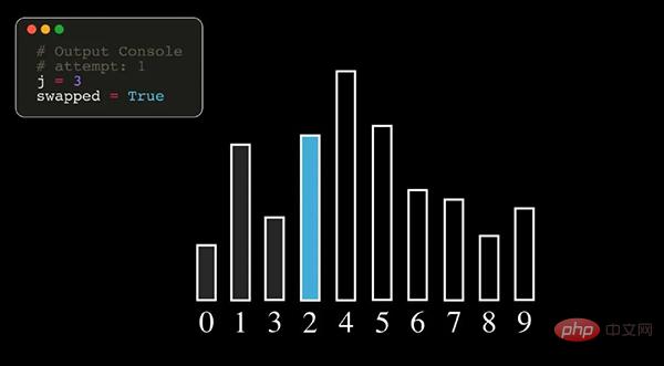
Note: In the above figure, the numbers represent the original index number of the data sequence.
Algorithm process
- Compare adjacent elements. If the former one is larger than the latter one, swap their positions.
- Do the same work for each pair of adjacent elements in the sorted array until all are completed. At this time, the last element will be the largest number in this round of sorting.
- Continue to repeat the above steps for the remaining elements until no element needs to be compared.
Bubble sorting finds the largest element each time, so it needs to be traversed n-1 times (n is the length of the data sequence).
Algorithm Features
When is the fastest (Best Cases): When the input data is already in positive sequence.
When is the slowest (Worst Cases): When the input data is in reverse order.
Python Code
def bubble_sort(lst):
n = len(lst)
for i in range(n):
for j in range(1, n - i):
if lst[j - 1] > lst[j]:
lst[j - 1], lst[j] = lst[j], lst[j - 1]
return lst
02 Selection Sort
Selection Sort Principle
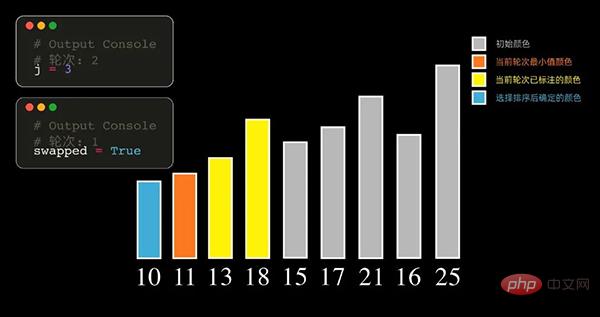
The principle of Selection Sort, each round starts from the records to be sorted Select the smallest element from the sequence and store it at the beginning of the sequence. Then find the smallest element from the remaining unsorted elements and put it at the end of the sorted sequence. And so on, until the number of all data elements to be sorted is zero. Get the data sequence sorted from the smallest arrival value.
You can also find the element with the largest value in each round. In this case, the sorted array will eventually be arranged from large to small.
Selection sort selects the smallest (largest) element each time, so it needs to be traversed n-1 times.
Python code
def selection_sort(lst):
for i in range(len(lst) - 1):
min_index = i
for j in range(i + 1, len(lst)):
if lst[j] < lst[min_index]:
min_index = j
lst[i], lst[min_index] = lst[min_index], lst[i]
return lst
03Quick Sort
Quick Sort (Quick Sort) was developed by Americans in the 1960s A sorting method proposed by Tony Hall. This sorting method was already a very fast sorting method at the time. Therefore, in terms of naming, it is called "quick sort".
Algorithm process
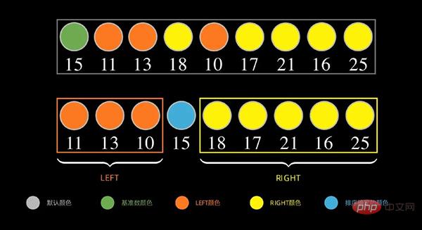
- First take a number from the data sequence as the baseline number (baseline, it is customary to take the first number).
- During the partitioning process, all numbers smaller than the base number are placed on its left side, and all numbers greater than or equal to it are placed on its right side.
- Repeat the second step recursively for the left and right intervals until there is only one number in each interval.
Because the order between data sequences is fixed. Finally, these subsequences are combined at once, and the overall sorting is completed.
As shown in the figure below, for the data sequence, first take the first data 15 as the base number, put the number smaller than 15 on the left, and the number larger than 15 (greater than or equal to) on the right
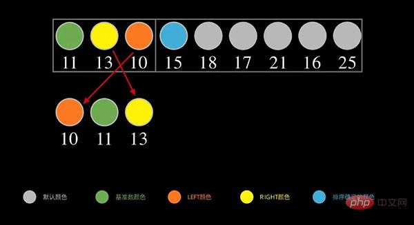
Next, for the left part, repeat the above steps, as shown below, take the first data 11 of the sequence on the left as the base number, and put the number smaller than 11 on the left. 11 Larger (greater than or equal to) numbers are placed on the right.
Continue to repeat the above process recursively until there is only one number in each interval. This will complete the sorting
Python code
def quick_sort(lst):
n = len(lst)
if n <= 1:
return lst
baseline = lst[0]
left = [lst[i] for i in range(1, len(lst)) if lst[i] < baseline]
right = [lst[i] for i in range(1, len(lst)) if lst[i] >= baseline]
return quick_sort(left) + [baseline] + quick_sort(right)
04Merge sort
Algorithm idea
Merge Sort (Merge Sort) is based on the merge operation An efficient sorting algorithm. This algorithm is a very typical application of the divide-and-conquer method. Merge sort merges two already ordered subsequences into an ordered sequence.
Algorithm process
Main two steps (split, merge)
- Step 1: Split the sequence until there is only one element;
- Step 2: After the split is completed, start the recursive merge.
Idea: Suppose we have an unsorted sequence, then we first use the splitting method to divide the sequence into sorted subsequences (until one element is left ). Then use the merge method to merge the ordered subsequences into an ordered sequence.
Graphic Algorithm
Split
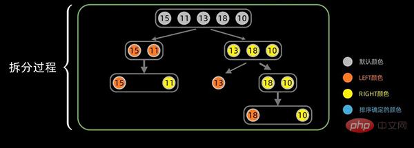
For the data sequence [15,11,13,18,10], we first start splitting from the middle position of the data sequence, The middle position is set to
and the first split is as follows:

第一次拆分后,依次对子序列进行拆分,拆分过程如下:
合并
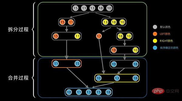
合并过程中,对于左右分区以及其子区间,递归使用合并方法。先从左边最小的子区间开始,对于每个区间,依次将最小的数据放在最左边,然后对右边区间也执行同样的操作。
合并过程的完整图示如下:
Python代码
def merge_sort(lst):
def merge(left,right):
i = 0
j = 0
result = []
while i < len(left) and j < len(right):
if left[i] <= right[j]:
result.append(left[i])
i += 1
else:
result.append(right[j])
j += 1
result = result + left[i:] + right[j:]
return result
n = len(lst)
if n <= 1:
return lst
mid = n // 2
left = merge_sort(lst[:mid])
right = merge_sort(lst[mid:])
return merge(left,right)
05堆排序
要理解堆排序(Heap Sort)算法,首先要知道什么是“堆”。
堆的定义
对于 n 个元素的数据序列
,当且仅当满足下列情形之一时,才称之为 堆:
情形1:

情形2:

若序列
是堆,则堆顶元素必为序列中n个元素的最小值或最大值。
小顶堆如下图所示:
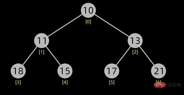
小顶堆
大顶堆如下图所示:
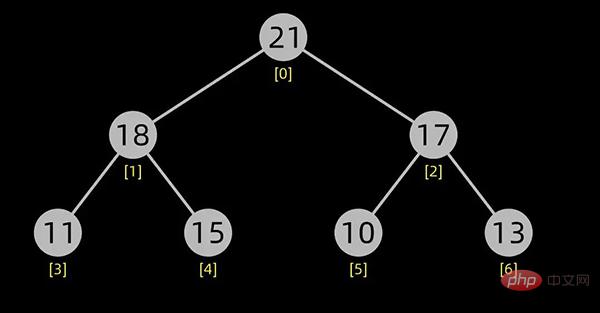
大顶堆
若在输出堆顶的最小值(或最大值)之后,使得剩余n-1个元素的序列重又建成一个堆,则得到n个元素的次小值(或次大值)。如此反复执行,便能得到一个有序序列,这个过程称之为 堆排序。
堆的存储
一般用数组来表示堆,若根结点存在序号 0 处, i 结点的父结点下标就为 (i-1)/2。i 结点的左右子结点下标分别为 2*i+1和 2*i+2 。
对于上面提到的小顶堆和大顶堆,其数据存储情况如下:
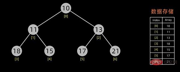
小顶堆
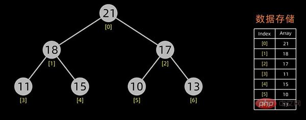
大顶堆
每幅图的右边为其数据存储结构,左边为其逻辑结构。
堆排序
实现堆排序需要解决两个问题:
- 如何由一个无序序列建成一个堆?
- 如何在输出堆顶元素之后,调整剩余元素成为一个新的堆?
堆的初始化
第一个问题实际上就是堆的初始化,下面来阐述下如何构造初始堆,假设初始的数据序列如下:

咱们首先需要将其以树形结构来展示,如下:
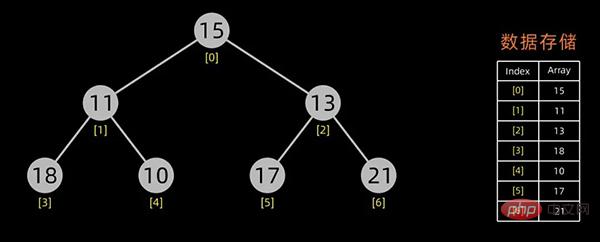
初始化堆的时候是对所有的非叶子结点进行筛选。
最后一个非终端元素的下标是 [n/2] 向下取整,所以筛选只需要从第 [n/2] 向下取整个元素开始,从后往前进行调整。
从最后一个非叶子结点开始,每次都是从父结点、左边子节点、右边子节点中进行比较交换,交换可能会引起子结点不满足堆的性质,所以每次交换之后需要重新对被交换的子结点进行调整。
以小顶堆为例,构造初始堆的过程如下:
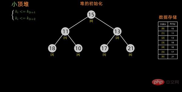
进行堆排序
有了初始堆之后就可以进行排序了。
堆排序是一种选择排序。建立的初始堆为初始的无序区。
排序开始,首先输出堆顶元素(因为它是最值),将堆顶元素和最后一个元素交换,这样,第n个位置(即最后一个位置)作为有序区,前n-1个位置仍是无序区,对无序区进行调整,得到堆之后,再交换堆顶和最后一个元素,这样有序区长度变为2。。。
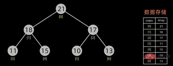
大顶堆
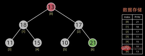
交换堆顶元素和最后的元素
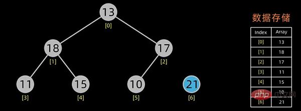
无序区-1,有序区+1
不断进行此操作,将剩下的元素重新调整为堆,然后输出堆顶元素到有序区。每次交换都导致无序区-1,有序区+1。不断重复此过程直到有序区长度增长为n-1,排序完成。
Python代码
def heap_sort(lst):
def adjust_heap(lst, i, size):
left_index = 2 * i + 1
right_index = 2 * i + 2
largest_index = i
if left_index < size and lst[left_index] > lst[largest_index]:
largest_index = left_index
if right_index < size and lst[right_index] > lst[largest_index]:
largest_index = right_index
if largest_index != i:
lst[largest_index], lst[i] = lst[i], lst[largest_index]
adjust_heap(lst, largest_index, size)
def built_heap(lst, size):
for i in range(len(lst)//2)[::-1]:
adjust_heap(lst, i, size)
size = len(lst)
built_heap(lst, size)
for i in range(len(lst))[::-1]:
lst[0], lst[i] = lst[i], lst[0]
adjust_heap(lst, 0, i)
return lst
06插入排序
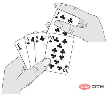
插入排序(Insertion Sort)就是每一步都将一个需要排序的数据按其大小插入到已经排序的数据序列中的适当位置,直到全部插入完毕。
插入排序如同打扑克牌一样,每次将后面的牌插到前面已经排好序的牌中。
Python代码
def insertion_sort(lst):
for i in range(len(lst) - 1):
cur_num, pre_index = lst[i+1], i
while pre_index >= 0 and cur_num < lst[pre_index]:
lst[pre_index + 1] = lst[pre_index]
pre_index -= 1
lst[pre_index + 1] = cur_num
return lst
07希尔排序
基本原理
希尔排序(Shell Sort)是插入排序的一种更高效率的实现。
希尔排序的核心在于间隔序列的设定。既可以提前设定好间隔序列,也可以动态的定义间隔序列。
这里以动态间隔序列为例来描述。初始间隔(gap值)为数据序列长度除以2取整,后续间隔以 前一个间隔数值除以2取整为循环,直到最后一个间隔值为 1 。
对于下面这个数据序列,初始间隔数值为5
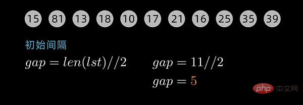
先将数据序列按间隔进行子序列分组,第一个子序列的索引为[0,5,10],这里分成了5组。

为方便大家区分不同的子序列,对同一个子序列标注相同的颜色,分组情况如下:
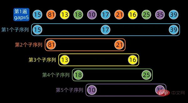
分组结束后,子序列内部进行插入排序,gap为5的子序列内部排序后如下:
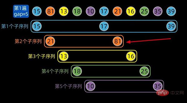

注:红色箭头标注的地方,是子序列内部排序后的状态
接下来选取第二个间隔值,按照间隔值进行子序列分组,同样地,子序列内部分别进行插入排序;
如果数据序列比较长,则会选取第3个、第4个或者更多个间隔值,重复上述的步骤。
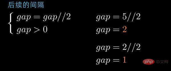
gap为2的排序情况前后对照如下:

最后一个间隔值为1,这一次相当于简单的插入排序。但是经过前几次排序,序列已经基本有序,因此最后一次排序时间效率就提高了很多。

Python代码
def shell_sort(lst):
n = len(lst)
gap = n // 2
while gap > 0:
for i in range(gap, n):
for j in range(i, gap - 1, -gap):
if lst[j] < lst[j - gap]:
lst[j], lst[j - gap] = lst[j - gap], lst[j]
else:
break
gap //= 2
return lst
08计数排序
基本原理
计数排序(Counting Sort)的核心在于将输入的数据值转化为键,存储在额外开辟的数组空间中。计数排序要求输入的数据必须是有确定范围的整数。
算法的步骤如下:
先找出待排序的数组中最大和最小的元素,新开辟一个长度为 最大值-最小值+1 的数组;
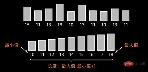
然后,统计原数组中每个元素出现的次数,存入到新开辟的数组中;
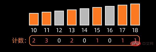
接下来,根据每个元素出现的次数,按照新开辟数组中从小到大的秩序,依次填充到原来待排序的数组中,完成排序。
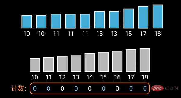
Python代码
def counting_sort(lst):
nums_min = min(lst)
bucket = [0] * (max(lst) + 1 - nums_min)
for num in lst:
bucket[num - nums_min] += 1
i = 0
for j in range(len(bucket)):
while bucket[j] > 0:
lst[i] = j + nums_min
bucket[j] -= 1
i += 1
return lst
09桶排序
基本思想
简单来说,桶排序(Bucket Sort)就是把数据分组,放在一个个的桶中,对每个桶里面的数据进行排序,然后将桶进行数据合并,完成桶排序。
该算法分为四步,包括划分桶、数据入桶、桶内排序、数据合并。
桶的划分过程
这里详细介绍下桶的划分过程。
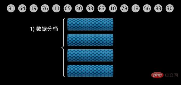
对于一个数值范围在10到 49范围内的数组,我们取桶的大小为10 (defaultBucketSize = 10),则第一个桶的范围为 10到20,第二个桶的数据范围是20到30,依次类推。最后,我们一共需要4个桶来放入数据。

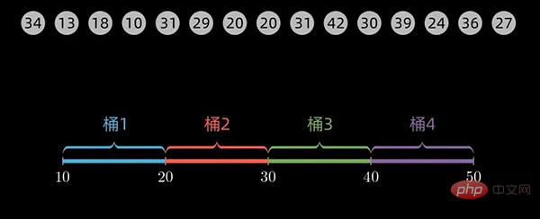
排序过程
对于下面这个数据序列,初始设定桶的大小为 20 (defaultBucketSize = 20),经计算,一共需要4个桶来放入数据。
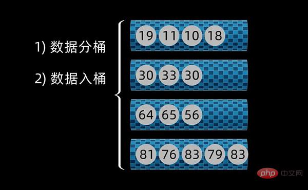
然后将原始数组按数值大小放入到对应的桶中,完成数据分组。
对于桶内的数据序列,这时可以用冒泡排序、选择排序等多种排序算法来对数据进行排序。这些算法,在之前的视频里已有介绍,大家可以去了解下。
这里,我选用 冒泡排序 来对桶内数据进行排序。
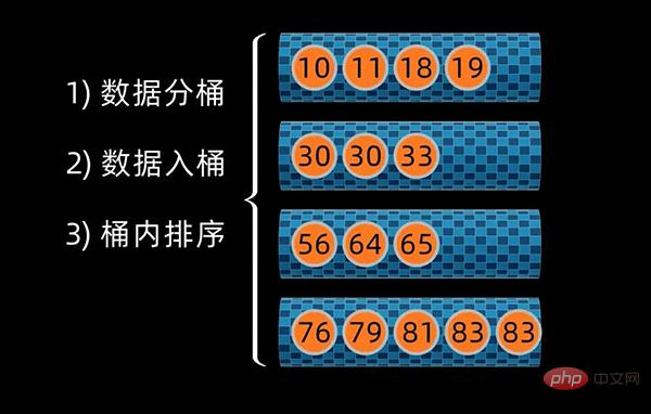
桶内排序完成后,将数据按桶的顺序进行合并,这样就得到所有数值排好序的数据序列了

Python代码
def bucket_sort(lst, defaultBucketSize=4):
maxVal, minVal = max(lst), min(lst)
bucketSize = defaultBucketSize
bucketCount = (maxVal - minVal) // bucketSize + 1
buckets = [[] for i in range(bucketCount)]
for num in lst:
buckets[(num - minVal) // bucketSize].append(num)
lst.clear()
for bucket in buckets:
bubble_sort(bucket)
lst.extend(bucket)
return lst
10基数排序
基数排序(radix sort)属于“分配式排序”(distribution sort),它是透过键值的部份信息,将要排序的元素分配至某些“桶”中,以达到排序的作用。
基数排序适用于所有元素均为正整数的数组。
基本思想
排序过程分为“分配”和“收集”。
排序过程中,将元素分层为多个关键码进行排序(一般按照数值的个位、十位、百位、…… 进行区分),多关键码排序按照从最主位关键码到最次位关键码或从最次位到最主位关键码的顺序逐次排序。
基数排序的方式可以采用最低位优先LSD(Least sgnificant digital)法或最高位优先MSD(Most sgnificant digital)法,LSD的排序方式由键值的最右边开始,而MSD则相反,由键值的最左边开始。
LSD的基数排序适用于位数小的数列,如果位数多的话,使用MSD的效率会比较好,MSD的方式恰与LSD相反,是由高位数为基底开始进行分配,其他的演算方式则都相同。
算法流程
这里以最低位优先LSD为例。
先根据个位数的数值,在扫描数值时将它们分配至编号0到9的桶中,然后将桶子中的数值串接起来。

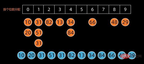
将这些桶子中的数值重新串接起来,成为新的序列,接着再进行一次分配,这次是根据十位数来分配。

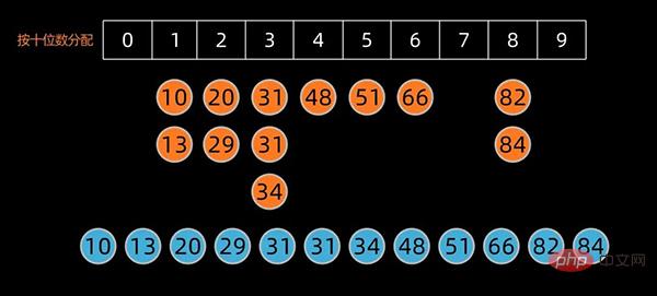
如果排序的对象有三位数以上,则持续进行以上的动作直至最高位数为止。
Python代码
# LSD Radix Sort
def radix_sort(lst):
mod = 10
div = 1
mostBit = len(str(max(lst)))
buckets = [[] for row in range(mod)]
while mostBit:
for num in lst:
buckets[num // div % mod].append(num)
i = 0
for bucket in buckets:
while bucket:
lst[i] = bucket.pop(0)
i += 1
div *= 10
mostBit -= 1
return lst
11小结
以上就是用 Python 来实现10种经典排序算法的相关内容。
对于这些排序算法的实现,代码其实并不是最主要的,重要的是需要去理解各种算法的基本思想、基本原理以及其内部的实现过程。
对于每种算法,用其他编程语言同样是可以去实现的。
并且,对于同一种算法,即使只用 Python 语言,也有多种不同的代码方式可以来实现,但其基本原理是一致的。
The above is the detailed content of Use Python to implement the top ten classic sorting algorithms. For more information, please follow other related articles on the PHP Chinese website!

Hot AI Tools

Undresser.AI Undress
AI-powered app for creating realistic nude photos

AI Clothes Remover
Online AI tool for removing clothes from photos.

Undress AI Tool
Undress images for free

Clothoff.io
AI clothes remover

AI Hentai Generator
Generate AI Hentai for free.

Hot Article

Hot Tools

Notepad++7.3.1
Easy-to-use and free code editor

SublimeText3 Chinese version
Chinese version, very easy to use

Zend Studio 13.0.1
Powerful PHP integrated development environment

Dreamweaver CS6
Visual web development tools

SublimeText3 Mac version
God-level code editing software (SublimeText3)

Hot Topics
 1385
1385
 52
52
 PHP and Python: Code Examples and Comparison
Apr 15, 2025 am 12:07 AM
PHP and Python have their own advantages and disadvantages, and the choice depends on project needs and personal preferences. 1.PHP is suitable for rapid development and maintenance of large-scale web applications. 2. Python dominates the field of data science and machine learning.
 Python vs. JavaScript: Community, Libraries, and Resources
Apr 15, 2025 am 12:16 AM
Python and JavaScript have their own advantages and disadvantages in terms of community, libraries and resources. 1) The Python community is friendly and suitable for beginners, but the front-end development resources are not as rich as JavaScript. 2) Python is powerful in data science and machine learning libraries, while JavaScript is better in front-end development libraries and frameworks. 3) Both have rich learning resources, but Python is suitable for starting with official documents, while JavaScript is better with MDNWebDocs. The choice should be based on project needs and personal interests.
 Detailed explanation of docker principle
Apr 14, 2025 pm 11:57 PM
Docker uses Linux kernel features to provide an efficient and isolated application running environment. Its working principle is as follows: 1. The mirror is used as a read-only template, which contains everything you need to run the application; 2. The Union File System (UnionFS) stacks multiple file systems, only storing the differences, saving space and speeding up; 3. The daemon manages the mirrors and containers, and the client uses them for interaction; 4. Namespaces and cgroups implement container isolation and resource limitations; 5. Multiple network modes support container interconnection. Only by understanding these core concepts can you better utilize Docker.
 How to run programs in terminal vscode
Apr 15, 2025 pm 06:42 PM
In VS Code, you can run the program in the terminal through the following steps: Prepare the code and open the integrated terminal to ensure that the code directory is consistent with the terminal working directory. Select the run command according to the programming language (such as Python's python your_file_name.py) to check whether it runs successfully and resolve errors. Use the debugger to improve debugging efficiency.
 Python: Automation, Scripting, and Task Management
Apr 16, 2025 am 12:14 AM
Python excels in automation, scripting, and task management. 1) Automation: File backup is realized through standard libraries such as os and shutil. 2) Script writing: Use the psutil library to monitor system resources. 3) Task management: Use the schedule library to schedule tasks. Python's ease of use and rich library support makes it the preferred tool in these areas.
 Is the vscode extension malicious?
Apr 15, 2025 pm 07:57 PM
VS Code extensions pose malicious risks, such as hiding malicious code, exploiting vulnerabilities, and masturbating as legitimate extensions. Methods to identify malicious extensions include: checking publishers, reading comments, checking code, and installing with caution. Security measures also include: security awareness, good habits, regular updates and antivirus software.
 What is vscode What is vscode for?
Apr 15, 2025 pm 06:45 PM
VS Code is the full name Visual Studio Code, which is a free and open source cross-platform code editor and development environment developed by Microsoft. It supports a wide range of programming languages and provides syntax highlighting, code automatic completion, code snippets and smart prompts to improve development efficiency. Through a rich extension ecosystem, users can add extensions to specific needs and languages, such as debuggers, code formatting tools, and Git integrations. VS Code also includes an intuitive debugger that helps quickly find and resolve bugs in your code.
 How to install nginx in centos
Apr 14, 2025 pm 08:06 PM
CentOS Installing Nginx requires following the following steps: Installing dependencies such as development tools, pcre-devel, and openssl-devel. Download the Nginx source code package, unzip it and compile and install it, and specify the installation path as /usr/local/nginx. Create Nginx users and user groups and set permissions. Modify the configuration file nginx.conf, and configure the listening port and domain name/IP address. Start the Nginx service. Common errors need to be paid attention to, such as dependency issues, port conflicts, and configuration file errors. Performance optimization needs to be adjusted according to the specific situation, such as turning on cache and adjusting the number of worker processes.


