
 Technology peripherals
AI
TabTransformer converter improves multi-layer perceptron performance in-depth analysis
Technology peripherals
AI
TabTransformer converter improves multi-layer perceptron performance in-depth analysis
TabTransformer converter improves multi-layer perceptron performance in-depth analysis

Today, Transformers are key modules in most advanced natural language processing (NLP) and computer vision (CV) architectures. However, the field of tabular data is still dominated by gradient boosted decision tree (GBDT) algorithms. So, there were attempts to bridge this gap. Among them, the first converter-based tabular data modeling paper is the paper "TabTransformer: Tabular Data Modeling Using Context Embedding" published by Huang et al. in 2020.
This article aims to provide a basic display of the content of the paper, while also delving into the implementation details of the TabTransformer model and showing you how to use TabTransformer specifically for our own data.
1. Paper Overview
The main idea of the above paper is that if a converter is used to convert conventional classification embeddings into contextual embeddings, then conventional multi-layer perception The performance of the processor (MLP) will be significantly improved. Next, let's understand this description in more depth.
1. Categorical Embeddings
In deep learning models, the classic way to use categorical features is to train their embeddings. This means that each category value has a unique dense vector representation and can be passed to the next layer. For example, you can see from the image below that each categorical feature is represented by a four-dimensional array. These embeddings are then concatenated with numerical features and used as input to the MLP.
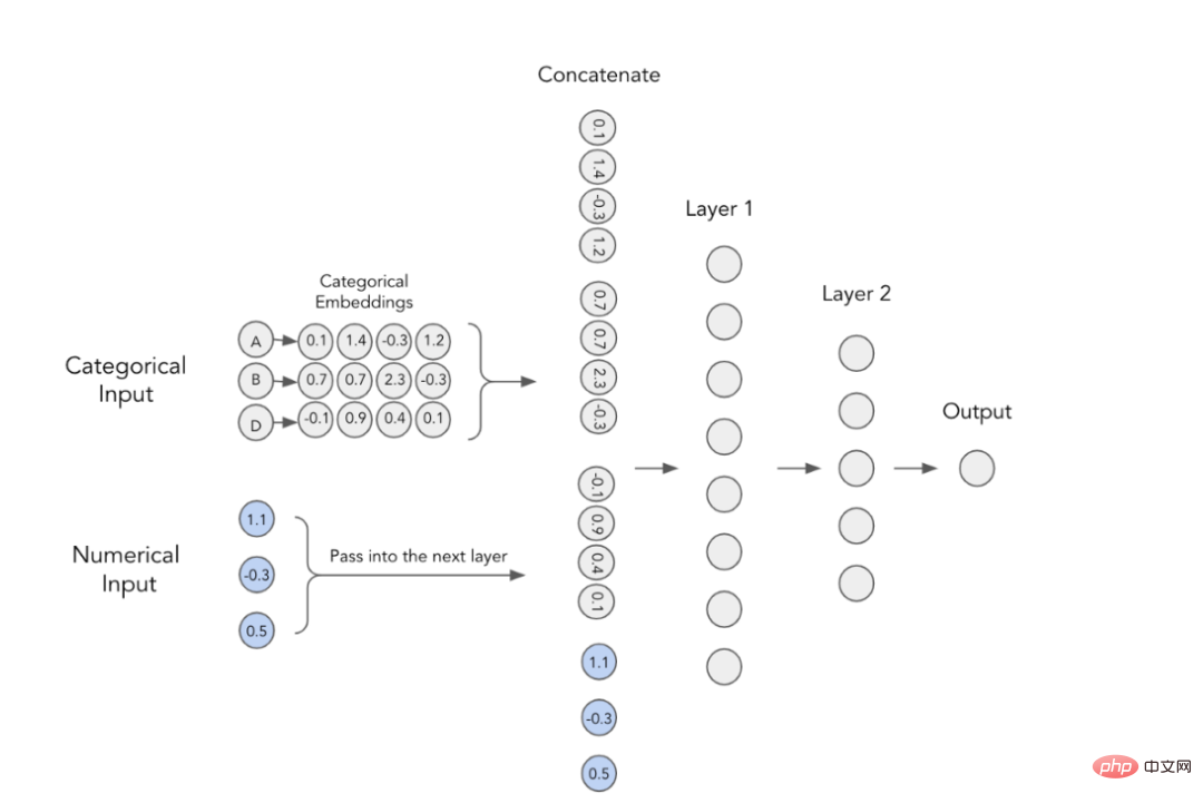
MLP with classification embedding
2. Contextual Embeddings
The authors of the paper believe that categorical embeddings lack contextual meaning, that is, they do not encode any interaction and relationship information between categorical variables. In order to make the embedded content more concrete, it has been suggested to use transformers currently used in the NLP field for this purpose.
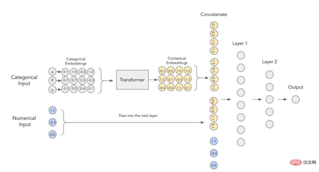
Context Embedding in TabTransformer Transformer
To visualize the above idea in a visual way, We might as well consider the following context embedding image obtained after training. Among them, two classification features are highlighted: relationship (black) and marital status (blue). These features are correlated; so the values for "Married," "Husband," and "Wife" should be close to each other in vector space, even though they come from different variables.
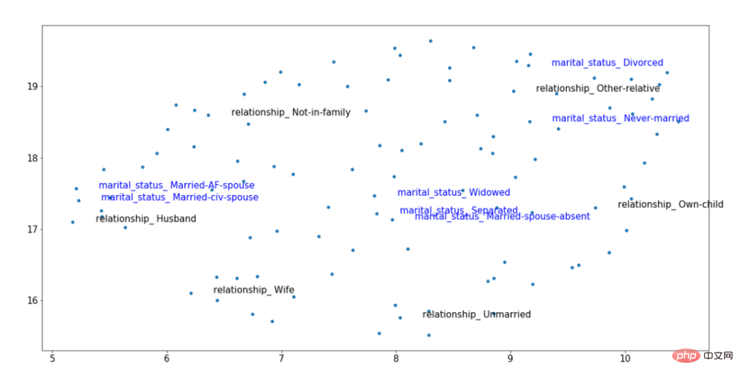
Example of embedding result of TabTransformer converter after training
Through the trained Context embedding results, we can see that the marital status of "Married" is closer to the relationship level of "Husband" and "Wife", while the classification of "non-married" The values come from a separate data cluster on the right. This type of context makes such embeddings more useful, an effect that is not possible using simple forms of category embedding techniques.
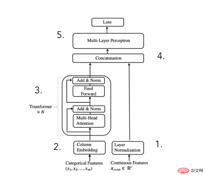
3.TabTransformer architecture
In order to achieve the above purpose, the author of the paper proposed the following architecture:
TabTransformer converter architecture diagram
(Excerpted from the paper published by Huang et al. in 2020)
We can This architecture is broken down into 5 steps:
- Standardize numeric features and pass them forward
- Embed categorical features
- Embedding passes N times Transformer block processing in order to obtain contextual embeddings
- Concatenate contextual categorical embeddings with numeric features
- Concatenate via MLP to obtain desired predictions
Although the model architecture is very simple, the authors of the paper stated that adding a converter layer can significantly improve computing performance. Of course, all the "magic" happens inside these converter blocks; so let's look at the implementation in more detail.
4. Converter
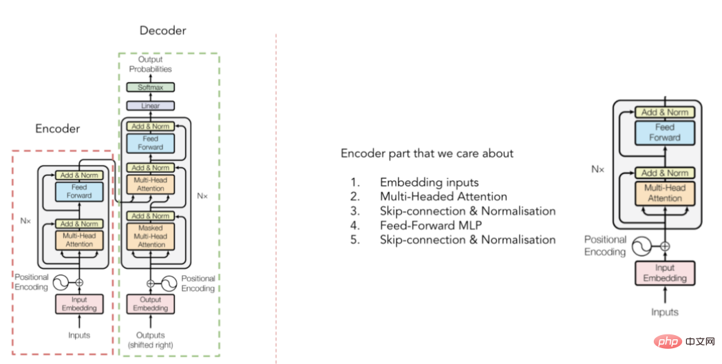
Transformer architecture diagram
(From Vaswani et al. 2017 paper)
You may have seen the converter architecture before, but for the sake of a quick introduction, remember that the converter is composed of an encoder It consists of two parts: the decoder and the decoder (see the figure above). For TabTransformer, we only care about the encoder part that contextualizes the input embeddings (the decoder part converts these embeddings into the final output result). But how exactly is it done? The answer is - multi-head attention mechanism.
5. Multi-head-attention mechanism
To quote a description from my favorite article on attention mechanisms, it goes like this:
“The key concept behind self-attention is that this mechanism allows The neural network learns how to schedule information with the best routing scheme between the various pieces of the input sequence."
In other words, self-attention helps the model Find out which parts of the input are more important and which parts are less important when representing a certain word/category. To that end, I highly recommend you read the article referenced above to get a more intuitive understanding of why self-focus is so effective.
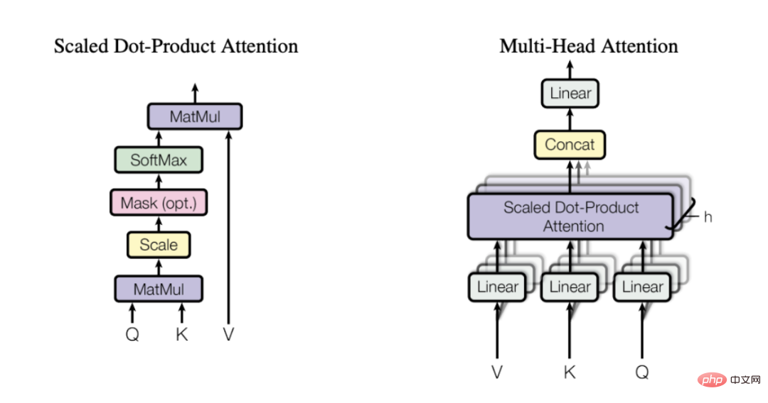
Multi-head attention mechanism
(selected from the paper published by Vaswani et al. in 2017)
Attention is calculated through 3 learned matrices - Q, K and V, which represent query (Query), key (Key) and value (Value). First, we multiply the matrices Q and K to get the attention matrix. This matrix is scaled and passed through the softmax layer. We then multiply this by the V matrix to get the final value. For a more intuitive understanding, consider the schematic below, which shows how we implement the transformation from input embedding to context embedding using matrices Q, K, and V.
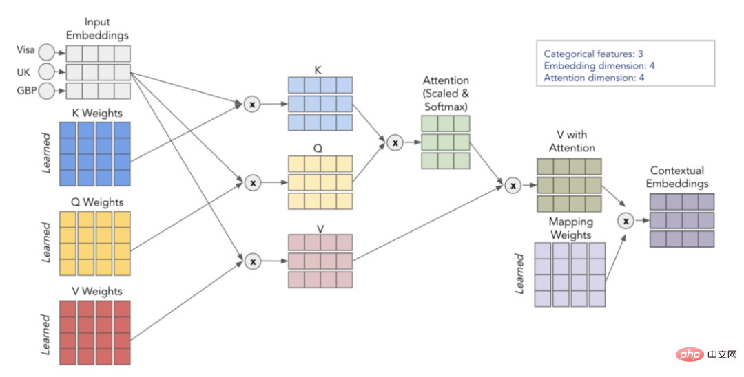
Visualization of self-focus process
By repeating the process h times (using different Q, K , V matrix), we can get multiple context embeddings, which form our final multi-head attention.
6. Brief review
Let us summarize what has been introduced above:
- Simple categorical embeddings do not contain contextual information
- By passing the categorical embeddings through the transformer encoder, we are able to contextualize the embeddings
- The transformer part is able to contextualize the embeddings because it A multi-head attention mechanism is used
- The multi-head attention mechanism uses matrices Q, K and V to find useful interaction and correlation information when encoding variables
- In TabTransformer, it is contextualized The embeddings are concatenated with numeric inputs and predicted through a simple MLP output
While the idea behind TabTransformer is simple, it may take you some time to master the attention mechanism . Therefore, I strongly recommend you to re-read the above explanation. If you're feeling a bit lost, read through all of the suggested links in this article. I guarantee that once you do this, it will not be difficult for you to understand how the attention mechanism works.
7. Experimental results display
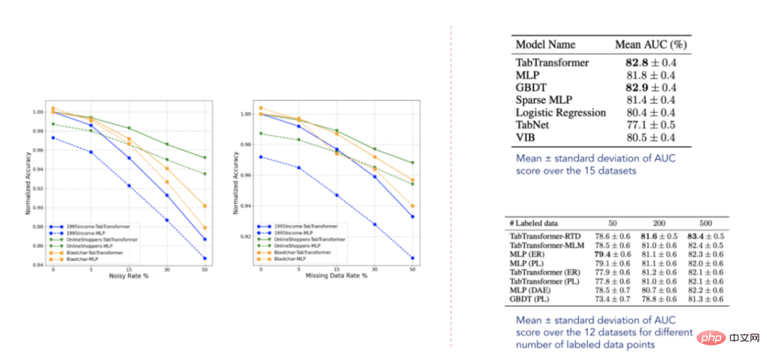
Result data (selected from Huang et al. 2020 Paper)
According to the reported results, TabTransformer outperforms all other deep learning tabular models, furthermore, it is close to the performance level of GBDT, which is very encouraging. The model is also relatively robust to missing and noisy data, and outperforms other models in semi-supervised settings. However, these datasets are clearly not exhaustive and there is still considerable room for improvement as confirmed by some related papers published in the future.
2. Build our own sample program
Now, let’s finally determine how to apply the model to our own data. The following example data is taken from the famous Tabular Playground Kaggle competition. To facilitate the use of the TabTransformer converter, I created a tabtransformertf package. It can be installed using the pip command like this:
pip install tabtransformertf
and allows us to use the model without extensive preprocessing.
1. Data preprocessing
The first step is to set the appropriate data type and convert our training and validation data to TF data set. Among them, the package installed earlier provides a good utility that can do this.
from tabtransformertf.utils.preprocessing import df_to_dataset, build_categorical_prep

# 设置数据类型
train_data[CATEGORICAL_FEATURES] = train_data[CATEGORICAL_FEATURES].astype(str)
val_data[CATEGORICAL_FEATURES] = val_data[CATEGORICAL_FEATURES].astype(str)

train_data[NUMERIC_FEATURES] = train_data[NUMERIC_FEATURES].astype(float)
val_data[NUMERIC_FEATURES] = val_data[NUMERIC_FEATURES].astype(float)

# 转换成TF数据集
train_dataset = df_to_dataset(train_data[FEATURES + [LABEL]], LABEL, batch_size=1024)
val_dataset = df_to_dataset(val_data[FEATURES + [LABEL]], LABEL, shuffle=False, batch_size=1024)
The next step is to prepare the preprocessing layer for the categorical data. This categorical data will later be passed to our main model.
from tabtransformertf.utils.preprocessing import build_categorical_prep

category_prep_layers = build_categorical_prep(train_data, CATEGORICAL_FEATURES)

# 输出结果是一个字典结构,其中键部分是特征名称,值部分是StringLookup层
# category_prep_layers ->
# {'product_code': <keras.layers.preprocessing.string_lookup.StringLookup at 0x7f05d28ee4e0>,
#'attribute_0': <keras.layers.preprocessing.string_lookup.StringLookup at 0x7f05ca4fb908>,
#'attribute_1': <keras.layers.preprocessing.string_lookup.StringLookup at 0x7f05ca4da5f8>}This is preprocessing! Now, we can start building the model.
2. Build the TabTransformer model
It’s easy to initialize the model. Among them, there are several parameters that need to be specified, but the most important parameters are: embedding_dim, depth and heads. All parameters are selected after hyperparameter tuning.
from tabtransformertf.models.tabtransformer import TabTransformer

tabtransformer = TabTransformer(
numerical_features = NUMERIC_FEATURES,# 带有数字特征名称的列表
categorical_features = CATEGORICAL_FEATURES, # 带有分类特征名称的列表
categorical_lookup=category_prep_layers, # 带StringLookup层的Dict
numerical_discretisers=None,# None代表我们只是简单地传递数字特征
embedding_dim=32,# 嵌入维数
out_dim=1,# Dimensionality of output (binary task)
out_activatinotallow='sigmoid',# 输出层激活
depth=4,# 转换器块层的个数
heads=8,# 转换器块中注意力头的个数
attn_dropout=0.1,# 在转换器块中的丢弃率
ff_dropout=0.1,# 在最后MLP中的丢弃率
mlp_hidden_factors=[2, 4],# 我们为每一层划分最终嵌入的因子
use_column_embedding=True,#如果我们想使用列嵌入,设置此项为真
)

# 模型运行中摘要输出:
# 总参数个数: 1,778,884
# 可训练的参数个数: 1,774,064
# 不可训练的参数个数: 4,820
After the model is initialized, we can install it like any other Keras model. Training parameters are also adjustable, so learning speed and early stopping can be adjusted at will.
LEARNING_RATE = 0.0001
WEIGHT_DECAY = 0.0001
NUM_EPOCHS = 1000

optimizer = tfa.optimizers.AdamW(
learning_rate=LEARNING_RATE, weight_decay=WEIGHT_DECAY
)

tabtransformer.compile(
optimizer = optimizer,
loss = tf.keras.losses.BinaryCrossentropy(),
metrics= [tf.keras.metrics.AUC(name="PR AUC", curve='PR')],
)

out_file = './tabTransformerBasic'
checkpoint = ModelCheckpoint(
out_file, mnotallow="val_loss", verbose=1, save_best_notallow=True, mode="min"
)
early = EarlyStopping(mnotallow="val_loss", mode="min", patience=10, restore_best_weights=True)
callback_list = [checkpoint, early]

history = tabtransformer.fit(
train_dataset,
epochs=NUM_EPOCHS,
validation_data=val_dataset,
callbacks=callback_list
)
3. Evaluation
The most critical indicator in the competition is ROC AUC. So, let’s output it together with the PR AUC metric to evaluate the model’s performance.
val_preds = tabtransformer.predict(val_dataset)

print(f"PR AUC: {average_precision_score(val_data['isFraud'], val_preds.ravel())}")
print(f"ROC AUC: {roc_auc_score(val_data['isFraud'], val_preds.ravel())}")

# PR AUC: 0.26
# ROC AUC: 0.58您也可以自己给测试集评分,然后将结果值提交给Kaggle官方。我现在选择的这个解决方案使我跻身前35%,这并不坏,但也不太好。那么,为什么TabTransfromer在上述方案中表现不佳呢?可能有以下几个原因:
- 数据集太小,而深度学习模型以需要大量数据著称
- TabTransformer很容易在表格式数据示例领域出现过拟合
- 没有足够的分类特征使模型有用
三、结论
本文探讨了TabTransformer背后的主要思想,并展示了如何使用Tabtransformertf包来具体应用此转换器。
归纳起来看,TabTransformer的确是一种有趣的体系结构,它在当时的表现明显优于大多数深度表格模型。它的主要优点是将分类嵌入语境化,从而增强其表达能力。它使用在分类特征上的多头注意力机制来实现这一点,而这是在表格数据领域使用转换器的第一个应用实例。
TabTransformer体系结构的一个明显缺点是,数字特征被简单地传递到最终的MLP层。因此,它们没有语境化,它们的价值也没有在分类嵌入中得到解释。在下一篇文章中,我将探讨如何修复此缺陷并进一步提高性能。
译者介绍
朱先忠,51CTO社区编辑,51CTO专家博客、讲师,潍坊一所高校计算机教师,自由编程界老兵一枚。
原文链接:https://towardsdatascience.com/transformers-for-tabular-data-tabtransformer-deep-dive-5fb2438da820?source=collection_home---------4----------------------------
The above is the detailed content of TabTransformer converter improves multi-layer perceptron performance in-depth analysis. For more information, please follow other related articles on the PHP Chinese website!

Hot AI Tools

Undresser.AI Undress
AI-powered app for creating realistic nude photos

AI Clothes Remover
Online AI tool for removing clothes from photos.

Undress AI Tool
Undress images for free

Clothoff.io
AI clothes remover

AI Hentai Generator
Generate AI Hentai for free.

Hot Article
Hot Tools

Notepad++7.3.1
Easy-to-use and free code editor

SublimeText3 Chinese version
Chinese version, very easy to use

Zend Studio 13.0.1
Powerful PHP integrated development environment

Dreamweaver CS6
Visual web development tools

SublimeText3 Mac version
God-level code editing software (SublimeText3)
Hot Topics
 1378
1378
 52
52

 This article will take you to understand SHAP: model explanation for machine learning
Jun 01, 2024 am 10:58 AM
This article will take you to understand SHAP: model explanation for machine learning
Jun 01, 2024 am 10:58 AM
In the fields of machine learning and data science, model interpretability has always been a focus of researchers and practitioners. With the widespread application of complex models such as deep learning and ensemble methods, understanding the model's decision-making process has become particularly important. Explainable AI|XAI helps build trust and confidence in machine learning models by increasing the transparency of the model. Improving model transparency can be achieved through methods such as the widespread use of multiple complex models, as well as the decision-making processes used to explain the models. These methods include feature importance analysis, model prediction interval estimation, local interpretability algorithms, etc. Feature importance analysis can explain the decision-making process of a model by evaluating the degree of influence of the model on the input features. Model prediction interval estimate
 Transparent! An in-depth analysis of the principles of major machine learning models!
Apr 12, 2024 pm 05:55 PM
Transparent! An in-depth analysis of the principles of major machine learning models!
Apr 12, 2024 pm 05:55 PM
In layman’s terms, a machine learning model is a mathematical function that maps input data to a predicted output. More specifically, a machine learning model is a mathematical function that adjusts model parameters by learning from training data to minimize the error between the predicted output and the true label. There are many models in machine learning, such as logistic regression models, decision tree models, support vector machine models, etc. Each model has its applicable data types and problem types. At the same time, there are many commonalities between different models, or there is a hidden path for model evolution. Taking the connectionist perceptron as an example, by increasing the number of hidden layers of the perceptron, we can transform it into a deep neural network. If a kernel function is added to the perceptron, it can be converted into an SVM. this one
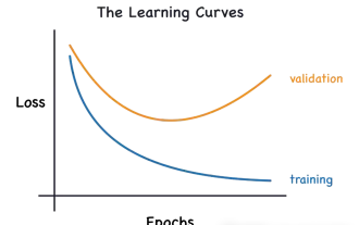 Identify overfitting and underfitting through learning curves
Apr 29, 2024 pm 06:50 PM
Identify overfitting and underfitting through learning curves
Apr 29, 2024 pm 06:50 PM
This article will introduce how to effectively identify overfitting and underfitting in machine learning models through learning curves. Underfitting and overfitting 1. Overfitting If a model is overtrained on the data so that it learns noise from it, then the model is said to be overfitting. An overfitted model learns every example so perfectly that it will misclassify an unseen/new example. For an overfitted model, we will get a perfect/near-perfect training set score and a terrible validation set/test score. Slightly modified: "Cause of overfitting: Use a complex model to solve a simple problem and extract noise from the data. Because a small data set as a training set may not represent the correct representation of all data." 2. Underfitting Heru
 The evolution of artificial intelligence in space exploration and human settlement engineering
Apr 29, 2024 pm 03:25 PM
The evolution of artificial intelligence in space exploration and human settlement engineering
Apr 29, 2024 pm 03:25 PM
In the 1950s, artificial intelligence (AI) was born. That's when researchers discovered that machines could perform human-like tasks, such as thinking. Later, in the 1960s, the U.S. Department of Defense funded artificial intelligence and established laboratories for further development. Researchers are finding applications for artificial intelligence in many areas, such as space exploration and survival in extreme environments. Space exploration is the study of the universe, which covers the entire universe beyond the earth. Space is classified as an extreme environment because its conditions are different from those on Earth. To survive in space, many factors must be considered and precautions must be taken. Scientists and researchers believe that exploring space and understanding the current state of everything can help understand how the universe works and prepare for potential environmental crises
 Implementing Machine Learning Algorithms in C++: Common Challenges and Solutions
Jun 03, 2024 pm 01:25 PM
Implementing Machine Learning Algorithms in C++: Common Challenges and Solutions
Jun 03, 2024 pm 01:25 PM
Common challenges faced by machine learning algorithms in C++ include memory management, multi-threading, performance optimization, and maintainability. Solutions include using smart pointers, modern threading libraries, SIMD instructions and third-party libraries, as well as following coding style guidelines and using automation tools. Practical cases show how to use the Eigen library to implement linear regression algorithms, effectively manage memory and use high-performance matrix operations.
 Explainable AI: Explaining complex AI/ML models
Jun 03, 2024 pm 10:08 PM
Explainable AI: Explaining complex AI/ML models
Jun 03, 2024 pm 10:08 PM
Translator | Reviewed by Li Rui | Chonglou Artificial intelligence (AI) and machine learning (ML) models are becoming increasingly complex today, and the output produced by these models is a black box – unable to be explained to stakeholders. Explainable AI (XAI) aims to solve this problem by enabling stakeholders to understand how these models work, ensuring they understand how these models actually make decisions, and ensuring transparency in AI systems, Trust and accountability to address this issue. This article explores various explainable artificial intelligence (XAI) techniques to illustrate their underlying principles. Several reasons why explainable AI is crucial Trust and transparency: For AI systems to be widely accepted and trusted, users need to understand how decisions are made
 Is Flash Attention stable? Meta and Harvard found that their model weight deviations fluctuated by orders of magnitude
May 30, 2024 pm 01:24 PM
Is Flash Attention stable? Meta and Harvard found that their model weight deviations fluctuated by orders of magnitude
May 30, 2024 pm 01:24 PM
MetaFAIR teamed up with Harvard to provide a new research framework for optimizing the data bias generated when large-scale machine learning is performed. It is known that the training of large language models often takes months and uses hundreds or even thousands of GPUs. Taking the LLaMA270B model as an example, its training requires a total of 1,720,320 GPU hours. Training large models presents unique systemic challenges due to the scale and complexity of these workloads. Recently, many institutions have reported instability in the training process when training SOTA generative AI models. They usually appear in the form of loss spikes. For example, Google's PaLM model experienced up to 20 loss spikes during the training process. Numerical bias is the root cause of this training inaccuracy,
 Five schools of machine learning you don't know about
Jun 05, 2024 pm 08:51 PM
Five schools of machine learning you don't know about
Jun 05, 2024 pm 08:51 PM
Machine learning is an important branch of artificial intelligence that gives computers the ability to learn from data and improve their capabilities without being explicitly programmed. Machine learning has a wide range of applications in various fields, from image recognition and natural language processing to recommendation systems and fraud detection, and it is changing the way we live. There are many different methods and theories in the field of machine learning, among which the five most influential methods are called the "Five Schools of Machine Learning". The five major schools are the symbolic school, the connectionist school, the evolutionary school, the Bayesian school and the analogy school. 1. Symbolism, also known as symbolism, emphasizes the use of symbols for logical reasoning and expression of knowledge. This school of thought believes that learning is a process of reverse deduction, through existing
